Weights in large scale assessments

In class, I’ve talked about using weights in large scale assessments. I’ve provided a bit of intuition about using weights and why they are important. Here’s some R syntax to go along with the example I discussed.

Imagine there are two schools in one school district. You are asked what is the average score on some measure of students in the district. There are only two schools (school A and B) and their size varies (School A = 100, School B = 1,000). You don’t have enough resources to assess everyone so you sample a total of 50 students (25 from each school).

First, create data for all the kids. This shows us the true state (which we don’t observe).

set.seed(123)
sa <- rnorm(100, 55, 2) #school A
sb <- rnorm(1000, 45, 2) #school B
district <- c(sa, sb) #district scores
hist(district, main = 'District Scores', xlab = 'Scores', breaks = 20)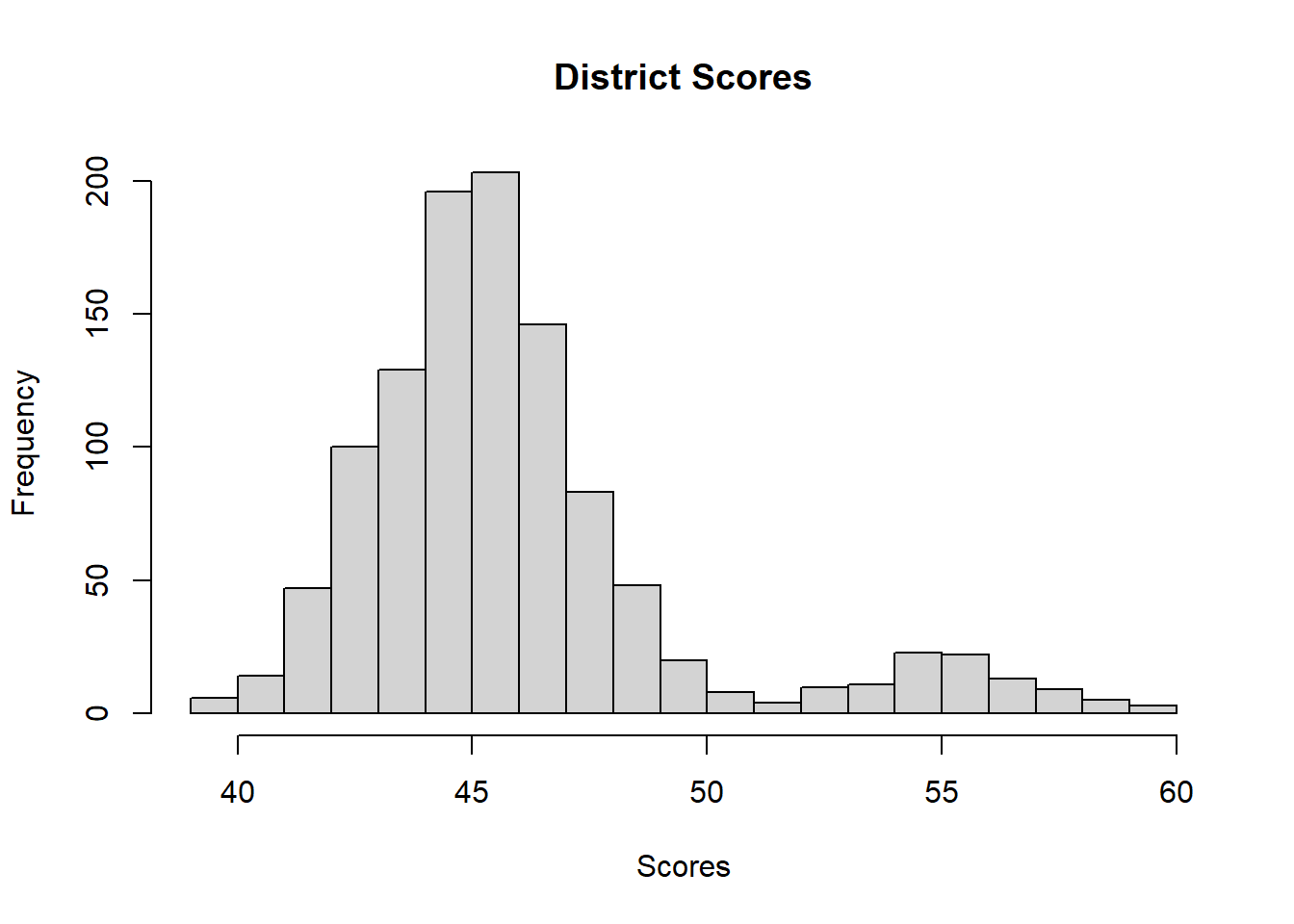

(ov <- mean(c(sa, sb))) #this is the true average score

[1] 45.96022

Now, imagine that we administer the assessment to 25 kids in each school:

sa.s <- sa[sample(100, 25)] #25 in school A
sb.s <- sb[sample(1000, 25)] #25 in school B

Here are the scores from each school. Close to the true means in each school:

mean(sa.s)

[1] 55.60827

mean(sb.s)

[1] 45.49553

If you merely take the average score of the 50 kids, this is not the mean of students in the school district:

(ov.s <- mean(c(sa.s, sb.s))) #not representative of the pop of interest

[1] 50.5519

But, we can use weights to make each response count appropriately. Remember weights are based on the inverse of the probability of selection. Let’s create a data.frame with this information:

sa.df <- data.frame(score = sa.s, wt = 1/(25/100), school = 'a')
sb.df <- data.frame(score = sb.s, wt = 1/(25/1000), school = 'b')
comb.df <- rbind(sa.df, sb.df)
psych::headTail(comb.df)

    score  wt school
1   54.72   4      a
2   56.56   4      a
3   59.34   4      a
4   55.61   4      a
...   ... ...   <NA>
47  44.47  40      b
48  47.76  40      b
49  44.03  40      b
50  45.21  40      b

You can see that the weights differ based on the school attended. Now, if we use the weights, we can make an estimate of what the average score is for the district:

weighted.mean(comb.df$score, comb.df$wt)

[1] 46.41487

sum(comb.df$wt) #summing the weights gives the population N

[1] 1100

Manually doing this:

((mean(sa.s) * 100) + (mean(sb.s) * 1000)) / 1100

[1] 46.41487

If we use a regression, just add the weights option. First, I show the results unweighted (this is just the mean of the 50 kids):

lm(score ~ 1, data = comb.df) #unweighted, not correct

Call:
lm(formula = score ~ 1, data = comb.df)

Coefficients:
(Intercept)  
      50.55  

If the weights option is used:

lm(score ~ 1, data = comb.df, weights = wt) #weighted

Call:
lm(formula = score ~ 1, data = comb.df, weights = wt)

Coefficients:
(Intercept)  
      46.41  

This is much closer the the true score. Using weights allows us to generalize to the population of interest.