Simulate some data

set.seed(123)
x <- rnorm(10, mean = 110, sd = 3) #make up some data
x

##  [1] 108.3186 109.3095 114.6761 110.2115 110.3879 115.1452 111.3827 106.2048
##  [9] 107.9394 108.6630

mean(x)

## [1] 110.2239

sd(x)

## [1] 2.861352

We have a vector with 10 elements. We can easily get the mean of this by just typing mean(x) but this is for illustrative purposes.

We create a likelihood function llike based on a normal distribution using:

\(f(x; \mu, \sigma^2) = \frac{1}{\sigma \sqrt{2\pi}}e^{-\frac{1}{2}(\frac{x - \mu}{\sigma})^2}\)

This take the sums of the log likelihood of whatever data is in x with a specified mean (mu) and standard deviation sigma– the later two we “don’t” know. There is also the built-in function of dnorm which we can use to check if we are getting the same results.

llike <- function(x, mu, sigma){
  sum(log((1 / (sigma * sqrt(2 * pi))) * exp(-.5 * ((x - mu) / sigma)^2)))
}

llike(x, 100, 10) #testing function to see if this works

## [1] -37.81005

#just checking if we specify m = 100, sd = 10
sum(dnorm(x, mean = 100, sd = 10, log = T)) #using built-in function

## [1] -37.81005

We get the same result using a specified mean of 100 and an SD of 10.

We can take a series of means (mu below) and see where the sum of the ll is at the highest.

mu <- seq(100, 120, .1) #set of values to test
ll <- sapply(mu, function(z)
  llike(x, z, 10) #find the log likelihood
)

plot(ll ~ mu) #plot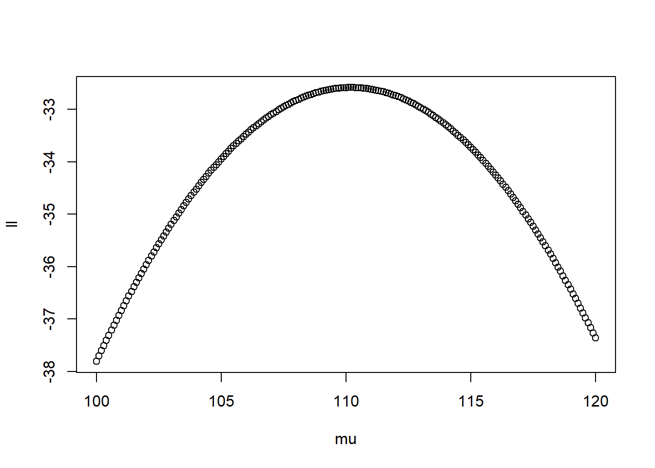 

mu[which(ll == max(ll))] #which mu had the highest point

## [1] 110.2

Based on the results, it peaks around 110.

We can use another function to find the maximum point (optimizing involves either finding the maximum or minimum). A lot of these ideas come from the very useful and accessible book of Hilbe and Robinson (2013) Methods of Statistical Model Estimation.

## another function to optimize
bb <- function(p, x){
  sum(dnorm(x, mean = p[1], sd = p[2], log = T))
}

## finding the maximum likelihood using 'optim'
fit <- optim(c(mean = 100, sd = 10), #starting values or guesses
      fn = bb, x = x,
      control = list(fnscale = -1)) #-1 to maximize
fit$par #contain the mean and the SD

##       mean         sd 
## 110.224295   2.715141

mean(x)

## [1] 110.2239

sd(x) #this is the actual variance

## [1] 2.861352

sqrt(sum((x - mean(x))^2) / length(x)) #this is the ML variance

## [1] 2.714517

# (SS / n), not n - 1
# based on ML
# the variance is under estimated

What about using ML in a regression?

I have not seen examples showing this. I’ve only seen examples of the first kind shown (e.g., getting the mean).

First, create some data with two variables (x1 and x2):

## simulate some data
set.seed(2468)
ns <- 1000
x1 <- rnorm(ns)
x2 <- rnorm(ns)
e1 <- rnorm(ns)
y <- 10 + 1 * x1 + .5 * x2 + e1
dat <- data.frame(y = y, x1 = x1, x2 = x2)

Prepare the formula and some matrices:

fml <- formula('y ~ x1 + x2')
df <- model.frame(fml, dat)
y <- model.response(df)
X <- model.matrix(fml, df)

Create another function to optimize:

## log likelihood for continuous variables
ll.cont <- function(p, X, y){
  len <- length(p)
  betas <- p
  mu <- X %*% betas
  sum((y - mu)^2) #minimize this, sum of squared residuals
}

In this case, we want to minimize the sums of squared residuals (error)– that’s what the best fitting line does.

start <- ncol(X) #how many start values
fit <- optim(p = rep(1, start), #repeat 1 
      fn = ll.cont, 
      X = X, y = y) #this minimizes the SSR
fit$par #compare with results below 

## [1] 9.9952812 1.0151535 0.5098497

## values are for the intercept / Bx1 / Bx2

Compare to using our standard lm function:

t1 <- lm(y ~ x1 + x2, data = df)
summary(t1)$coef

##              Estimate Std. Error   t value      Pr(>|t|)
## (Intercept) 9.9950936 0.03144700 317.83937  0.000000e+00
## x1          1.0153582 0.03116854  32.57638 4.166280e-159
## x2          0.5096043 0.03093340  16.47424  4.091831e-54

Instead of minimizing the error, what if we want to maximize the likelihoods again?

ll.cont.mx <- function(p, X, y){
  len <- length(p)
  betas <- p[-len]
  mu <- X %*% betas
  sds <- p[len]
  sum(dnorm(y, mean = mu, sd = sds, log = T)) #maximize this
  #sum((y - mu)^2) #minimize this
}

start <- ncol(X) + 1 #add one w/c is the variance
fit <- optim(p = rep(1, start), #starting values
             fn = ll.cont.mx, #function to use
             X = X, y = y, #pass this to our
             hessian = T, #to get standard errors
             control = list(fnscale = -1, #to maximize
             reltol = 1e-10) #change in deviance to converge
)
b <- fit$par[1:3] #the betas
ll <- fit$value #the log likelihood
conv <- fit$convergence #value of zero means convergence
ses <- sqrt(diag(solve(-fit$hessian)))[1:3] #get the SE from the inverse of the Hessian matrix
df <- data.frame(b, ses, t = b/ses)       
rownames(df) <- colnames(X)
df #putting it all together   

##                     b        ses         t
## (Intercept) 9.9951172 0.03139866 318.32944
## x1          1.0153670 0.03112063  32.62681
## x2          0.5095777 0.03088585  16.49874

ll #the log likelihood

## [1] -1411.179

t1 <- lm(y ~ x1 + x2, data = df)
summary(t1)$coef

##              Estimate Std. Error   t value      Pr(>|t|)
## (Intercept) 9.9950936 0.03144700 317.83937  0.000000e+00
## x1          1.0153582 0.03116854  32.57638 4.166280e-159
## x2          0.5096043 0.03093340  16.47424  4.091831e-54

logLik(t1)

## 'log Lik.' -1411.179 (df=4)

Similar coefficients, standard errors, and the same log likelihood.

— END