1. Estimating the OLS model using matrices
As a starting point, just begin with using an OLS model and estimating the results using different matrices. The standard ordinary least squares model (OLS) can be written as: \(y = XB + \varepsilon\) where \(X\) is a design matrix, \(B\) is a column vector of coefficents, plus some random error \(\varepsilon\).
Of interest is \(B\) which is obtained through: \(B = (X'X)^{-1}(X'y)\). For example (compare results using matrices and just using the coef function):
ols1 <- lm(mpg ~ wt + am, data = mtcars) #toy example
X <- model.matrix(ols1)
y <- mtcars$mpg
(betas <- solve(t(X) %*% X) %*% t(X) %*% y)
## [,1]
## (Intercept) 37.32155131
## wt -5.35281145
## am -0.02361522coef(ols1)## (Intercept) wt am
## 37.32155131 -5.35281145 -0.02361522The variance/covariance matrix of the betas, \(Var(\hat{\beta})\), of which the square root of the diagonal is the standard error, is: \(\sigma^2(X'X)^{-1}\). \(\sigma^2\) is based on the residuals and the residuals are merely the observed value less the predicted value:
modres <- residuals(ols1)
modres2 <- y - X %*% betas #manual computation
## compare
head(modres)
## Mazda RX4 Mazda RX4 Wag Datsun 710 Hornet 4 Drive
## -2.2735701 -0.9086032 -2.0794135 1.2877375
## Hornet Sportabout Valiant
## -0.2078799 -0.7008237head(modres2)## [,1]
## Mazda RX4 -2.2735701
## Mazda RX4 Wag -0.9086032
## Datsun 710 -2.0794135
## Hornet 4 Drive 1.2877375
## Hornet Sportabout -0.2078799
## Valiant -0.7008237\(\sigma^2\) is the sum of squared residuals divided by \(N - k\) where k is the number of predictors (including the intercept).
sigma(ols1)^2 #just using a function## [1] 9.597231n <- nobs(ols1)
k <- ols1$rank
sum(modres^2) / (n - k) #manual computation## [1] 9.597231The sum of squared residuals can be computed using \(u'u\) where \(u\) contains the residuals. (we use as.numeric to convert it into a scalar that we can use to multiply later on).
u <- modres2
(sigma2 <- as.numeric(t(u) %*% u / (n - k)))
## [1] 9.597231#manual computation using matricesUsing \(\sigma^2\), we can obtain the variance/covariance matrix:
(vcm <- sigma2 * solve(t(X) %*% X)) #manual computation## (Intercept) wt am
## (Intercept) 9.330816 -2.3417207 -3.6849277
## wt -2.341721 0.6213282 0.8436983
## am -3.684928 0.8436983 2.3890195vcov(ols1) #compare when using a function## (Intercept) wt am
## (Intercept) 9.330816 -2.3417207 -3.6849277
## wt -2.341721 0.6213282 0.8436983
## am -3.684928 0.8436983 2.3890195The square root of the diagonal is the standard error. Can compare to the results using the lm function.
se <- sqrt(diag(vcm))
tstat <- betas / se
pval <-  2 * pt(-abs(tstat), df = n - k)
data.frame(betas, se, tstat, pval)
## betas se tstat pval
## (Intercept) 37.32155131 3.0546385 12.21799285 5.843477e-13
## wt -5.35281145 0.7882438 -6.79080719 1.867415e-07
## am -0.02361522 1.5456453 -0.01527855 9.879146e-01summary(ols1)$coefficients #compare results## Estimate Std. Error t value Pr(>|t|)
## (Intercept) 37.32155131 3.0546385 12.21799285 5.843477e-13
## wt -5.35281145 0.7882438 -6.79080719 1.867415e-07
## am -0.02361522 1.5456453 -0.01527855 9.879146e-012. Using matrices to reconstruct the mixed model coefficients
Note, the procedure outlined below does not estimate the coefficients- which is done using an iterative process. The steps below merely reconstruct the mixed model coefficients given the already estimated elements.
For mixed models (a.k.a. multilevel models, hierarchical linear models, random coefficient models), this can be expressed as: \(y = X\beta + Zb + \varepsilon\). The difference is the presence of the random effects terms which use \(Zb\). \(Z\) is an \(n \times q\) design matrix of random effects where \(q\) is the number of random effects. \(b\) is a \(q \times 1\) vector of random effects.1 Sometimes \(b\) is shown as \(u\) but I used \(u\) already to represent the residuals so didn’t want to mix that up.
Using the bdf dataset in the mlmRev package, we can use the lmer function in lme4. There are 2,287 students from 131 schools.
library(lme4)
data(bdf, package = 'mlmRev')
mlm1 <- lmer(aritPOST ~ aritPRET + sex +
 schoolSES + (sex | schoolNR), data = bdf)
With a random intercept model, there is only one (q = 1) random effect. With a random coefficient model (in this case sex), we have two (q = 2). We just specified in this example that slopes can randomly vary by sex. NOTE: this function (as written) only works if the original data is sorted by the clustering variable and there is no missing data. That’s not an assumption for mixed models, just a limitation of my presentation/syntax. If you need to sort your data by the clusterid, can use dat <- dat[order(dat$cluster), ].
# The data are sorted by cluster already
X <- model.matrix(mlm1) #the design matrix
B <- fixef(mlm1) #to extract the coefficients from lme4-- just as a check, don't use it here
y <- mlm1@resp$y #outcome
Z <- getME(mlm1, 'Z') #sparse Z design matrix
b <- getME(mlm1, 'b') #random effects
Gname <- names(getME(mlm1, 'l_i')) #name of clustering variable
js <- table(mlm1@frame[, Gname]) #how many observation in each cluster
\(Z\) is a sparse matrix (just zeroes in the off diagonal).
qq <- getME(mlm1, 'q') #columns in Z matrix
NG <- ngrps(mlm1)
nre <- getME(mlm1, 'p_i') #qq/NG --> number of random effects
inde <- cumsum(js) #number per group summed to create an index
cols <- seq(1, (NG * nre), by = nre) #dynamic columns for Z matrix.
#if a random intercept model, cols is only a sequence from 1
#to NG
G <- bdiag(VarCorr(mlm1)) #G matrix
\(G\) is the variance/covariance matrix of the random effects (estimated using lmer). The following is used to create the \(V\) matrix, Probably other (better and faster) ways to to do this but I think this is the most “transparent” and works. The coefficients in actuality are estimated using an iterative process (which is different from the approach using OLS).
ml <- list() #empty list to store matricesThe ml object is an empty list of matrices. The following creates a matrix of \(ZGZ' + r\) for each cluster. \(G\) is the covariance matrix for the random effects– this matrix is used several times (and is just one matrix).
G## 2 x 2 sparse Matrix of class "dgCMatrix"
## (Intercept) sex1
## (Intercept) 4.9241939 -0.3289331
## sex1 -0.3289331 0.9752748If a random intercept model, \(G\) is a single number only. If there is one random slope, this becomes a \(2 \times 2\) matrix. \(r\) is composed of the a diagonal matrix with the residual variance (sigma(mlm1)^2) on the diagonal.
for (i in 1:NG){

    if (i == 1) { #if first cluster
      st = 1} else { #start at row 1
        st = inde[i - 1] + 1}

    end = st + js[i] - 1

    nc <- cols[i]
    ncend <- cols[i] + (nre - 1)

Zi <- Z[st:end, nc:ncend] #depends on how many obs in a cluster and
# how many rand effects
ml[[i]] <- Zi %*% G %*% t(Zi) + diag(sigma(mlm1)^2, nrow = js[i]) #ZGZ' + r
}
Each cluster/group has its own matrix. For example, cluster 2 has 7 observations and cluster 3 has 5 observations. This indicates how large the matrix is for those clusters.
Elements of matrix 2 and 3 in the list (which is cluster 2 and 3):
ml[[2]] #for the second cluster## 7 x 7 sparse Matrix of class "dgCMatrix"
## 26 27 28 29 30 31 32
## 26 24.930147 4.595261 4.595261 5.241602 4.595261 5.241602 4.595261
## 27 4.595261 24.612739 4.924194 4.595261 4.924194 4.595261 4.924194
## 28 4.595261 4.924194 24.612739 4.595261 4.924194 4.595261 4.924194
## 29 5.241602 4.595261 4.595261 24.930147 4.595261 5.241602 4.595261
## 30 4.595261 4.924194 4.924194 4.595261 24.612739 4.595261 4.924194
## 31 5.241602 4.595261 4.595261 5.241602 4.595261 24.930147 4.595261
## 32 4.595261 4.924194 4.924194 4.595261 4.924194 4.595261 24.612739ml[[3]] #for the third cluster## 5 x 5 sparse Matrix of class "dgCMatrix"
## 33 34 35 36 37
## 33 24.612739 4.924194 4.595261 4.595261 4.595261
## 34 4.924194 24.612739 4.595261 4.595261 4.595261
## 35 4.595261 4.595261 24.930147 5.241602 5.241602
## 36 4.595261 4.595261 5.241602 24.930147 5.241602
## 37 4.595261 4.595261 5.241602 5.241602 24.930147We can use the bdiag function to create a block diagonal matrix which accepts a list of matrices as an input. This ml is used to create a V matrix.
Vm <- bdiag(ml) #makes a block diagonal weighting matrix
image(Vm) #shows that this is a sparse matrix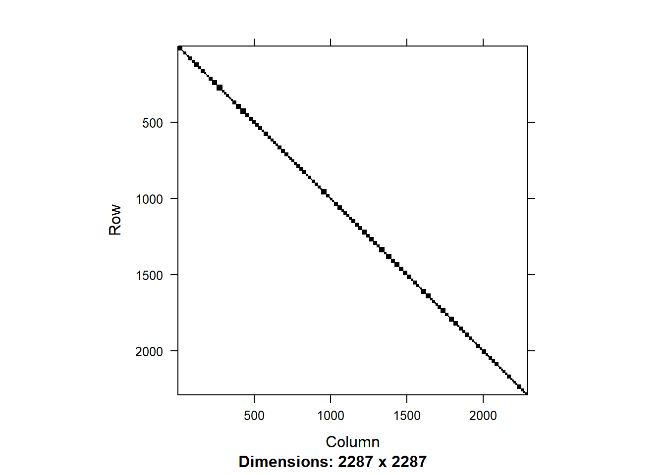
\(Vm\) is a block diagonal (sparse) matrix (V matrix). This matrix is used when computing the gamma coefficients and standard errors.
If using nlme, can extract the matrices using a function to put together the \(V\) matrix. This is actually simpler using:
### THIS IS JUST IF THE MODEL IS ESTIMATED USING LME
### NOT RUN IN THIS EXAMPLE

ml <- list()
for (j in 1:NG){
  test <- getVarCov(mlm1, individuals = j, type = 'marginal')
  ml[[j]] <- test[[1]]
}

Vm <- bdiag(ml)
For the fixed effects: \((X'V^{-1}X)^{-1} X'V^{-1}y\).
gammas <- solve(t(X) %*% solve(Vm) %*% X) %*% (t(X) %*% solve(Vm) %*% y)
gammas #manually computed using existing matrices
## 4 x 1 Matrix of class "dgeMatrix"
## [,1]
## [1,] 1.2277854
## [2,] 1.1250565
## [3,] -0.8269814
## [4,] 0.2660345fixef(mlm1) #using the mlm object## (Intercept) aritPRET sex1 schoolSES
## 1.2277854 1.1250565 -0.8269814 0.2660345The variance/covariance matrix (used to get the standard errors) is: \((X'V^{-1}X)^{-1}\)
mlm.vc <- solve(t(X) %*% solve(Vm) %*% X)
mlm.vc #manual computation
## 4 x 4 Matrix of class "dgeMatrix"
## [,1] [,2] [,3] [,4]
## [1,] 0.966855981 -0.0083507665 -0.0195023895 -0.0437988235
## [2,] -0.008350766 0.0008909363 0.0001694822 -0.0001181135
## [3,] -0.019502389 0.0001694822 0.0449218913 -0.0001316506
## [4,] -0.043798823 -0.0001181135 -0.0001316506 0.0024375222vcov(mlm1) #automatic## 4 x 4 Matrix of class "dpoMatrix"
## (Intercept) aritPRET sex1 schoolSES
## (Intercept) 0.966855981 -0.0083507665 -0.0195023895 -0.0437988235
## aritPRET -0.008350766 0.0008909363 0.0001694822 -0.0001181135
## sex1 -0.019502389 0.0001694822 0.0449218913 -0.0001316506
## schoolSES -0.043798823 -0.0001181135 -0.0001316506 0.0024375222Putting this together:
gammas <- as.numeric(gammas)
mlm.se <- as.numeric(sqrt(diag(mlm.vc)))
tstat <- gammas / mlm.se
data.frame(vars = names(fixef(mlm1)), estimate = gammas, se = mlm.se, t = tstat)
## vars estimate se t
## 1 (Intercept) 1.2277854 0.98328835 1.248652
## 2 aritPRET 1.1250565 0.02984856 37.692159
## 3 sex1 -0.8269814 0.21194785 -3.901816
## 4 schoolSES 0.2660345 0.04937127 5.388447summary(mlm1)$coef## Estimate Std. Error t value
## (Intercept) 1.2277854 0.98328835 1.248652
## aritPRET 1.1250565 0.02984856 37.692159
## sex1 -0.8269814 0.21194785 -3.901816
## schoolSES 0.2660345 0.04937127 5.388447Results are the same.