Creating grayscale images using PCA
The following links were helpful: 1. https://cran.r-project.org/web/packages/imager/vignettes/gettingstarted.html 2. https://stats.stackexchange.com/questions/229092/how-to-reverse-pca-and-reconstruct-original-variables-from-several-principal-com
library(tidyverse) #for ggplot, %>%
library(imager) #to read in the jpg

image1 <- load.image("C:/Users/huangf/Box Sync/Fun/snorlax/01_data/snorlax_g2.jpg")
Can download the image from: http://faculty.missouri.edu/huangf/data/snorlax_g2.jpg
Somehow is not reading directly from the website… To view the image
plot(image1)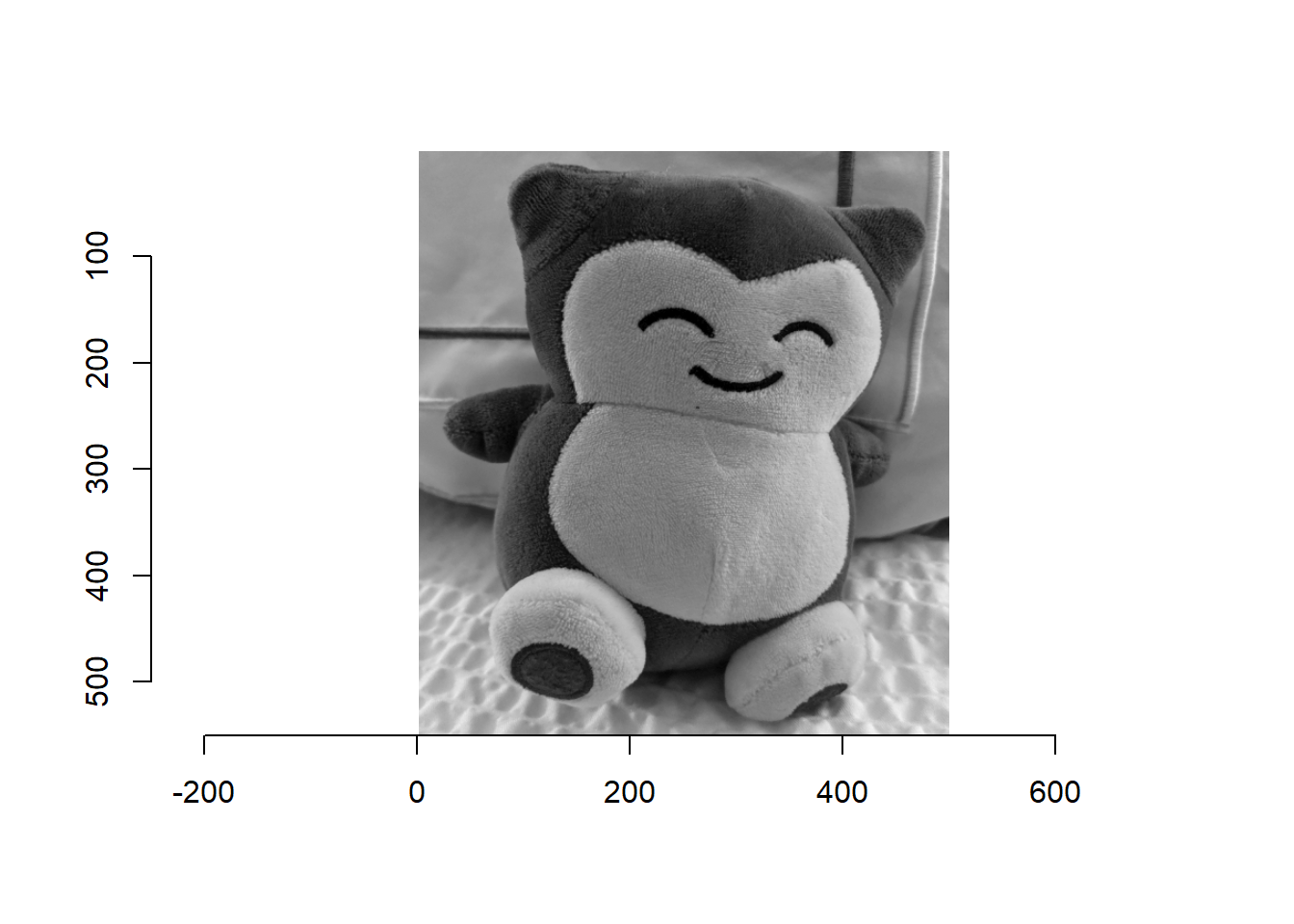
## NOTE 0,0 is in the upper left corner

image1
## Image. Width: 500 pix Height: 550 pix Depth: 1 Colour channels: 1dim(image1)## [1] 500 550 1 1#500 x 550 pixels
xwidth = dim(image1)[1] #just saving these
yheight = dim(image1)[2]
dat <- as.data.frame(image1) #create a tall dataset
#that can work with ggplot
head(dat)## x y value
## 1 1 1 0.5137255
## 2 2 1 0.5058824
## 3 3 1 0.5098039
## 4 4 1 0.5137255
## 5 5 1 0.5098039
## 6 6 1 0.5098039### plotting the image
ggplot(dat, aes(x = x, y = y, fill = value)) +
geom_raster() + theme_bw() +
scale_fill_gradient(low = "black", high = "white")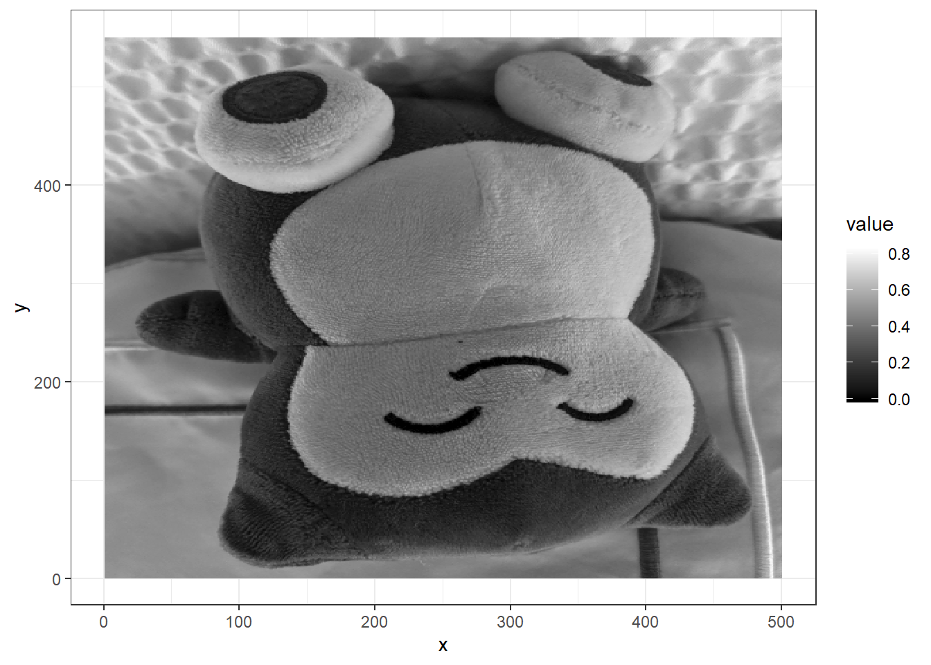
### NOTE: 0, 0 is in the lower left corner so we
### should just flip it

ggplot(dat, aes(x = x, y = y, fill = value)) +
  geom_raster() + theme_bw() +
  scale_y_reverse() +  #add to flip scale
  scale_fill_gradient(low = "black", high = "white")
OK, so we know the image renders correctly, let’s experiment using PCA.
First, create a wide data frame to use in a PCA.
Preparing to run the PCA
wide <- pivot_wider(dat, id_cols = x,
 names_from = 'y', names_prefix = 'y',
 values_from = 'value')
dim(wide) #just checking
## [1] 500 551wide[1:5, 1:5] #just checking## # A tibble: 5 x 5
## x y1 y2 y3 y4
## <int> <dbl> <dbl> <dbl> <dbl>
## 1 1 0.514 0.510 0.510 0.510
## 2 2 0.506 0.506 0.510 0.514
## 3 3 0.510 0.506 0.514 0.510
## 4 4 0.514 0.510 0.510 0.502
## 5 5 0.510 0.514 0.510 0.506wide2 <- select(wide, -x) #just remove x variable
wide2[1:5, 1:5]## # A tibble: 5 x 5
## y1 y2 y3 y4 y5
## <dbl> <dbl> <dbl> <dbl> <dbl>
## 1 0.514 0.510 0.510 0.510 0.510
## 2 0.506 0.506 0.510 0.514 0.506
## 3 0.510 0.506 0.514 0.510 0.510
## 4 0.514 0.510 0.510 0.502 0.510
## 5 0.510 0.514 0.510 0.506 0.506Running a PCA (manually)
cvm <- cov(wide2) #using covariance matrix :: you can use the
## correlation matrix but the scaling will be different (since it's standardized)
ev <- eigen(cvm)
str(ev) #has both eigen values and eigen vectors
## List of 2
## $ values : num [1:550] 4.583 2.479 0.832 0.609 0.568 ...
## $ vectors: num [1:550, 1:550] 0.00565 0.00565 0.00571 0.00578 0.00528 ...
## - attr(*, "class")= chr "eigen"evalues <- ev$values
loadings <- ev$vectors
mus <- colMeans(wide2) #need this later when we return to original
zwide <- scale(wide2, center = T, scale = F) #need this for
#principal component scores, just centered, not scaled
## principal component scores
pcs <- as.matrix(zwide) %*% loadings
cor(pcs)[1:5, 1:5] %>% round #not correlated (as it should be)## [,1] [,2] [,3] [,4] [,5]
## [1,] 1 0 0 0 0
## [2,] 0 1 0 0 0
## [3,] 0 0 1 0 0
## [4,] 0 0 0 1 0
## [5,] 0 0 0 0 1head(pcs)[1:5, 1:5]## [,1] [,2] [,3] [,4] [,5]
## [1,] 2.922521 0.2774740 -0.8150739 -0.2730839 -0.9014217
## [2,] 2.929396 0.2661346 -0.8064723 -0.2990911 -0.8866691
## [3,] 2.956576 0.2717294 -0.7936503 -0.3144499 -0.8792177
## [4,] 2.980215 0.2632674 -0.7617172 -0.3190132 -0.8769835
## [5,] 2.999131 0.2674471 -0.7381271 -0.3130517 -0.8847785# plot(evalues) #scree plot, if interested, but we have 500+
# so just limit to first 20
plot(evalues[1:20], type = 'b',
ylab = 'eigenvalues',
xlab = 'Prin Component #') #scree plot, if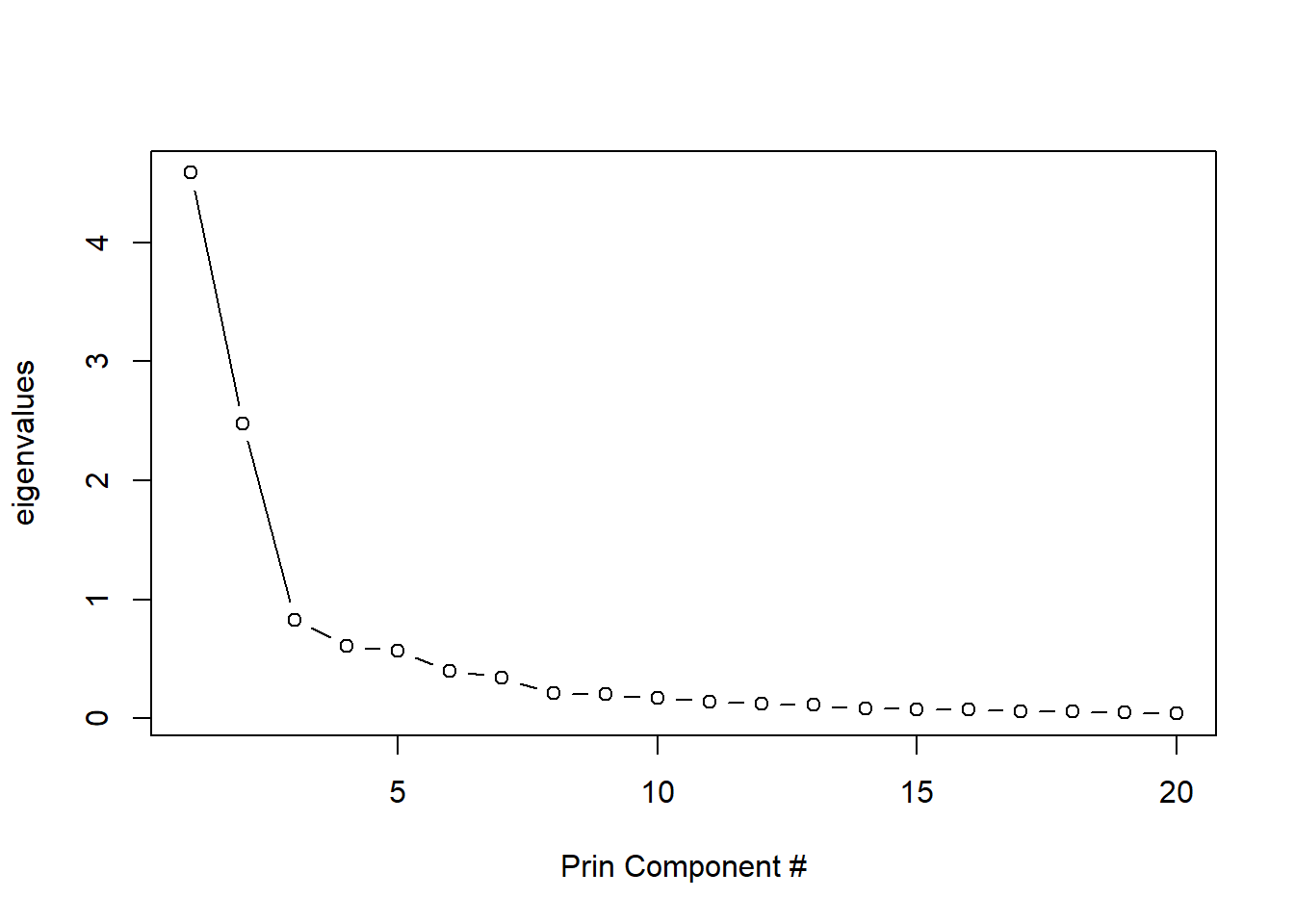
#what percent do first 10 eigenvalues each account for in variance?
(evalues / sum(evalues))[1:10]
## [1] 0.38328068 0.20726950 0.06958218 0.05089264 0.04747089 0.03365118
## [7] 0.02876539 0.01757143 0.01710983 0.01435288(evalues / sum(evalues))[1:10] %>% sum #90% of variance## [1] 0.8699466Creating original data using all component scores & loadings
tmp <- pcs %*% t(loadings) #component scores x loadings
tmp2 <- scale(tmp, center = -mus, scale = F) #reintroduce mean
head(tmp2)[1:5, 1:5] #reconstituted
## [,1] [,2] [,3] [,4] [,5]
## [1,] 0.5137255 0.5098039 0.5098039 0.5098039 0.5098039
## [2,] 0.5058824 0.5058824 0.5098039 0.5137255 0.5058824
## [3,] 0.5098039 0.5058824 0.5137255 0.5098039 0.5098039
## [4,] 0.5137255 0.5098039 0.5098039 0.5019608 0.5098039
## [5,] 0.5098039 0.5137255 0.5098039 0.5058824 0.5058824head(wide)[1:5, 1:5] #original data frame## # A tibble: 5 x 5
## x y1 y2 y3 y4
## <int> <dbl> <dbl> <dbl> <dbl>
## 1 1 0.514 0.510 0.510 0.510
## 2 2 0.506 0.506 0.510 0.514
## 3 3 0.510 0.506 0.514 0.510
## 4 4 0.514 0.510 0.510 0.502
## 5 5 0.510 0.514 0.510 0.506### place the matrix into a data frame
new2 <- data.frame(tmp2)
names(new2) <- 1:yheight #add names, just numbers (coordinates)
new2$x <- row.names(new2) %>% as.numeric #add x coordinate
tall2 <- pivot_longer(new2, 1:yheight, names_to = 'y') #create tall
tall2$y <- as.numeric(tall2$y) #when pivoting, y because a character
ggplot(tall2, aes(x = x, y = y, fill = value)) +
geom_raster() + theme_bw() + scale_y_reverse() +
scale_fill_gradient(low = "black", high = "white")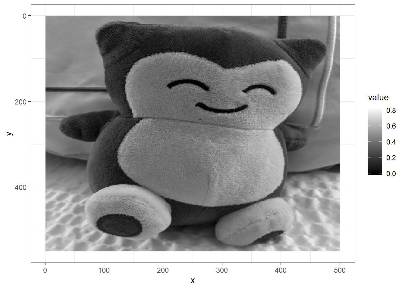
So what if we just use the first 10 components? (out of 500+)
ncomp <- 10 #number of components to use
### Creating data using 10 components
tmp <- pcs[,1:ncomp] %*% t(loadings[,1:ncomp]) #component scores x loadings
tmp2 <- scale(tmp, center = -mus, scale = F) #add back mean
head(tmp2)[1:5, 1:5] #reconstituted
## [,1] [,2] [,3] [,4] [,5]
## [1,] 0.5494325 0.5454111 0.5435424 0.5449286 0.5446933
## [2,] 0.5488673 0.5449852 0.5431840 0.5445829 0.5443818
## [3,] 0.5484028 0.5446355 0.5428195 0.5441641 0.5439251
## [4,] 0.5473589 0.5438008 0.5420109 0.5433143 0.5430735
## [5,] 0.5473990 0.5438387 0.5419770 0.5432045 0.5429343head(wide)[1:5, 1:5] #original data frame## # A tibble: 5 x 5
## x y1 y2 y3 y4
## <int> <dbl> <dbl> <dbl> <dbl>
## 1 1 0.514 0.510 0.510 0.510
## 2 2 0.506 0.506 0.510 0.514
## 3 3 0.510 0.506 0.514 0.510
## 4 4 0.514 0.510 0.510 0.502
## 5 5 0.510 0.514 0.510 0.506new2 <- data.frame(tmp2)
names(new2) <- 1:yheight #add names
new2$x <- row.names(new2) %>% as.numeric #add x coordinate
tall2 <- pivot_longer(new2, 1:yheight, names_to = 'y') #create tall
tall2$y <- as.numeric(tall2$y) #when pivoting, y because a character
ggplot(tall2, aes(x = x, y = y, fill = value)) +
geom_raster() + theme_bw() + labs(y = '') + scale_y_reverse() +
scale_fill_gradient(low = "black", high = "white") 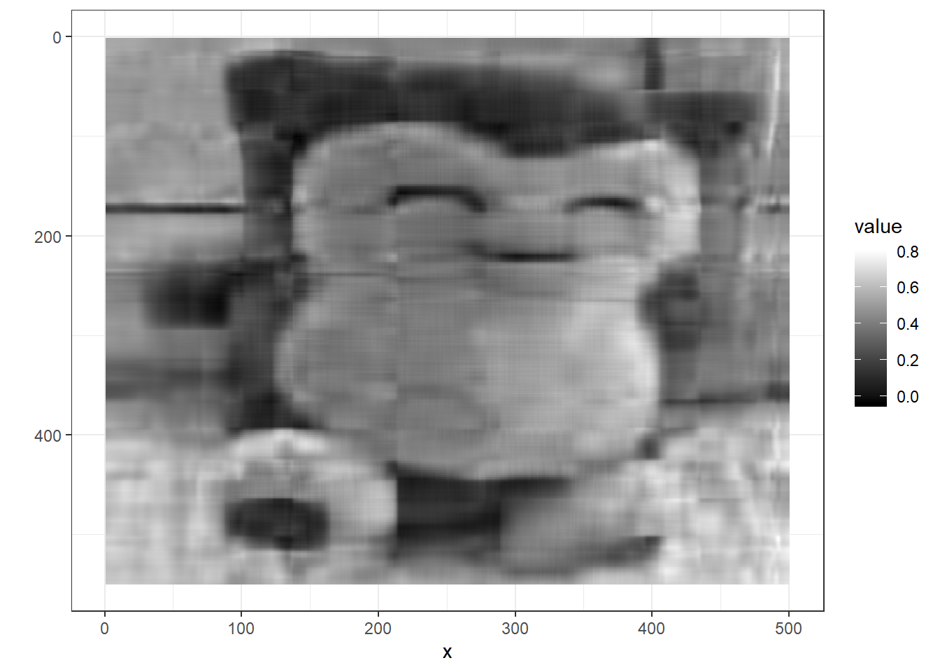
Image is not very clear!
What if we use more components?
ncomp <- 40 #number of components to use
tmp <- pcs[,1:ncomp] %*% t(loadings[,1:ncomp]) #component scores x loadings
tmp2 <- scale(tmp, center = -mus, scale = F) #add back mean
### place the matrix into a data frame
new2 <- data.frame(tmp2)
names(new2) <- 1:yheight #add names
new2$x <- row.names(new2) %>% as.numeric #add x coordinate
tall2 <- pivot_longer(new2, 1:yheight, names_to = 'y') #create tall
tall2$y <- as.numeric(tall2$y) #when pivoting, y because a character
ggplot(tall2, aes(x = x, y = y, fill = value)) +
  geom_raster() + theme_bw() + labs(y = '') + scale_y_reverse() +
scale_fill_gradient(low = "black", high = "white") 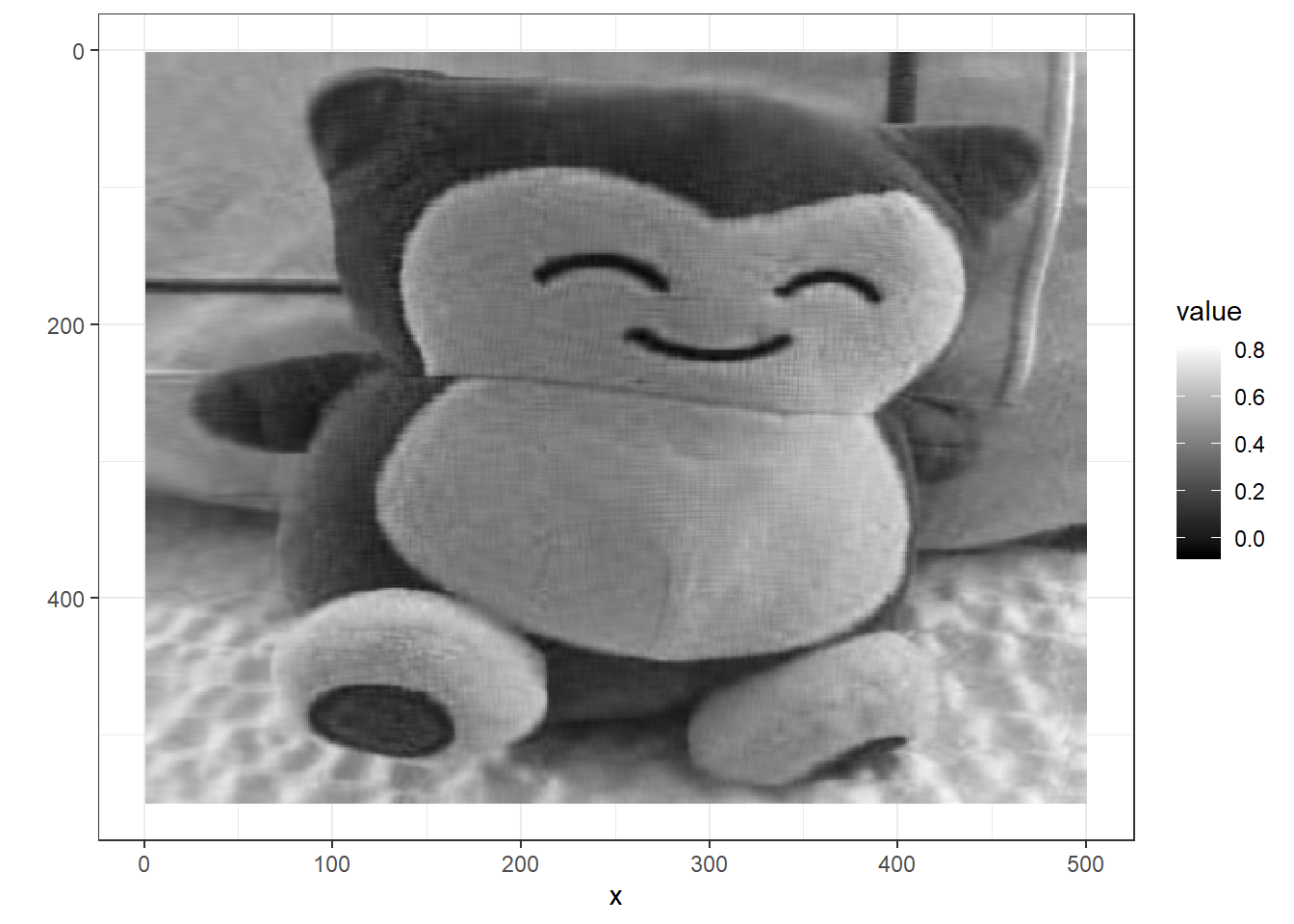
Much clearer image with 40 components (out of 500+)
Using Base R and prcomp
Got this from: https://kieranhealy.org/blog/archives/2019/10/27/reconstructing-images-using-pca/
img_pca <- prcomp(wide2)
im <- summary(img_pca)
im$importance[,1:10] #compare with manual computation
## PC1 PC2 PC3 PC4 PC5
## Standard deviation 2.140883 1.574353 0.9121861 0.7801209 0.753439
## Proportion of Variance 0.383280 0.207270 0.0695800 0.0508900 0.047470
## Cumulative Proportion 0.383280 0.590550 0.6601300 0.7110200 0.758500
## PC6 PC7 PC8 PC9 PC10
## Standard deviation 0.6343583 0.5865021 0.458393 0.452332 0.4142896
## Proportion of Variance 0.0336500 0.0287700 0.017570 0.017110 0.0143500
## Cumulative Proportion 0.7921500 0.8209100 0.838480 0.855590 0.8699500names(img_pca)## [1] "sdev" "rotation" "center" "scale" "x"dim(img_pca$x) #component scores## [1] 500 500dim(img_pca$rotation) #loadings (just the eigenvectors)## [1] 550 500img_pca$rotation[1:5, 1:5]## PC1 PC2 PC3 PC4 PC5
## y1 -0.005650860 0.01864489 0.010587733 -0.02943221 0.05041304
## y2 -0.005645269 0.02003725 0.008689557 -0.02681190 0.04938164
## y3 -0.005712267 0.02144366 0.007472650 -0.02769441 0.04921155
## y4 -0.005784892 0.02284957 0.006774656 -0.02926209 0.05068930
## y5 -0.005280473 0.02349464 0.006134465 -0.03049060 0.05210808ev$vectors[1:5, 1:5] #our original## [,1] [,2] [,3] [,4] [,5]
## [1,] 0.005650860 -0.01864489 -0.010587733 -0.02943221 -0.05041304
## [2,] 0.005645269 -0.02003725 -0.008689557 -0.02681190 -0.04938164
## [3,] 0.005712267 -0.02144366 -0.007472650 -0.02769441 -0.04921155
## [4,] 0.005784892 -0.02284957 -0.006774656 -0.02926209 -0.05068930
## [5,] 0.005280473 -0.02349464 -0.006134465 -0.03049060 -0.05210808####
new <- img_pca$x[, 1:xwidth] %*% t(img_pca$rotation)
new <- scale(new, center = -mus, scale = F)
new2 <- data.frame(new)
new2[1:5, 1:5]## y1 y2 y3 y4 y5
## 1 0.5137255 0.5098039 0.5098039 0.5098039 0.5098039
## 2 0.5058824 0.5058824 0.5098039 0.5137255 0.5058824
## 3 0.5098039 0.5058824 0.5137255 0.5098039 0.5098039
## 4 0.5137255 0.5098039 0.5098039 0.5019608 0.5098039
## 5 0.5098039 0.5137255 0.5098039 0.5058824 0.5058824names(new2) <- 1:yheight
dim(new2)## [1] 500 550new2$x <- row.names(new2) %>% as.numeric
tall2 <- pivot_longer(new2, 1:yheight)
tall2$y <- as.numeric(tall2$name)
ggplot(tall2, aes(x = x, y = y, fill = value)) +
geom_raster() + scale_y_reverse() + theme_bw() +
labs(y = '') +
scale_fill_gradient(low = "black", high = "white")