Notes for students. International large scale assessments (ILSAs) have several characteristics that should be accounted for to generate correct results. The characteristics that are important to account for include: 1) the use of plausible values; 2) the use of weights; and 3) the cluster sampling used. Some of the datasets that this applies to include TIMSS, PISA, PIRLS, and even NAEP (not international). Certain packages can also be used (e.g., intsvy, EdSurvey) but I just show how to “manually” calculate the results. I have noticed several articles that say that you can take one plausible value or just average the plausible values– these are incorrect (you can work with 1 PV in an exploratory manner though). Those articles also cite some documentation from the OECD but the complete paragraph in the OECD manual states that all the PVs should be used.
Weights and clustering can be accounted for by (of course) 1) using the provided weights, and 2) the clustering can be accounted for by using multilevel modeling or cluster robust standard errors. However, plausible values require the data to be analyzed \(m\) number of times and the data combined appropriately (using Rubin’s rules). In other words, the data are combined using the same rules as when multiply imputed datasets are combined. The point estimates are merely averaged though the standard errors need to take into account various additional sources of variance (i.e., do not merely average the standard errors in the datasets).
library(lme4)
library(dplyr)
library(tidyr) #to convert to tall format

#NOTE: The tall dataset is also downloadable in the next section...

l1 <- rio::import('http://faculty.missouri.edu/huangf/data/timss2015/STU_USA_2018.sav')
l2 <- rio::import('http://faculty.missouri.edu/huangf/data/timss2015/SCH_USA_2018.sav')
names(l1) <- tolower(names(l1))
names(l2) <- tolower(names(l2))

l1_ <- select(l1, starts_with("bsmm"),parent_ed, idstud,
              books, likemath, stuwgt, totwgt, idschool)
l2_ <- select(l2, schwgt, sch_ses, ag_parent_ed, idschool)
comb <- merge(l1_, l2_, by = 'idschool')
comb2 <- na.omit(comb) #merge l1 and l2
comb2$nwt <- comb2$totwgt / mean(comb2$totwgt) #normalized weights
####
names(comb2)
[1] "idschool" "bsmmat01" "bsmmat02" "bsmmat03" "bsmmat04"
[6] "bsmmat05" "parent_ed" "idstud" "books" "likemath"
[11] "stuwgt" "totwgt" "schwgt" "sch_ses" "ag_parent_ed"
[16] "nwt" dim(comb2)[1] 5688 16head(comb2) idschool bsmmat01 bsmmat02 bsmmat03 bsmmat04 bsmmat05 parent_ed idstud books
1 1 514.4249 505.7916 519.7016 531.0448 542.1232 4 10301 1
2 1 587.6541 579.3172 562.0366 550.9720 568.2771 4 10302 2
3 1 582.5530 553.8961 568.8929 601.2752 561.2372 1 10303 1
4 1 507.9202 501.7667 498.4307 504.9045 499.1313 4 10304 1
5 1 534.9643 547.8417 530.0570 555.7876 541.7867 4 10305 2
6 1 465.7001 466.2036 471.4720 455.1264 495.3281 3 10306 2
likemath stuwgt totwgt schwgt sch_ses ag_parent_ed nwt
1 2 4.704543 191.4986 40.70502 1 2.612903 0.5394655
2 1 4.704543 191.4986 40.70502 1 2.612903 0.5394655
3 2 4.704543 191.4986 40.70502 1 2.612903 0.5394655
4 2 4.704543 191.4986 40.70502 1 2.612903 0.5394655
5 1 4.704543 191.4986 40.70502 1 2.612903 0.5394655
6 1 4.704543 191.4986 40.70502 1 2.612903 0.5394655IMPORTANT NOTE: this dataset is a reduced sample of the TIMSS USA 2015 dataset. Do not use this for your own studies– this is just used for demonstration purposes.
Because of the plausible values (there are five listed per observations) all beginning with bsmmat (for math), these have to be converted into a tall dataset- where there are five datasets created with each observation having only one of the (imputed) plausible values. The regression are done 5 times, once per dataset, and the results combined.
## convert to tall using tidyr
tall <- tidyr::pivot_longer(comb2, starts_with("bsmm"),
                     values_to = 'math',
                     names_to = '.imp')
names(tall)
[1] "idschool" "parent_ed" "idstud" "books" "likemath"
[6] "stuwgt" "totwgt" "schwgt" "sch_ses" "ag_parent_ed"
[11] "nwt" ".imp" "math" dim(tall) #dimensions[1] 28440 13table(tall$.imp) #that variable .imp indicates w/c PV was used
bsmmat01 bsmmat02 bsmmat03 bsmmat04 bsmmat05
    5688     5688     5688     5688     5688
# NOTE: the tall dataset can be downloaded here
# tall <- rio::import("http://faculty.missouri.edu/huangf/data/talltimss.csv")
head(tall, n = 5) # A tibble: 5 x 13
idschool parent_ed idstud books likemath stuwgt totwgt schwgt sch_ses
<dbl> <dbl> <dbl> <dbl> <dbl> <dbl> <dbl> <dbl> <dbl>
1 1 4 10301 1 2 4.70 191. 40.7 1
2 1 4 10301 1 2 4.70 191. 40.7 1
3 1 4 10301 1 2 4.70 191. 40.7 1
4 1 4 10301 1 2 4.70 191. 40.7 1
5 1 4 10301 1 2 4.70 191. 40.7 1
# ... with 4 more variables: ag_parent_ed <dbl>, nwt <dbl>, .imp <chr>,
# math <dbl>tall is now a long/tall dataset. However, this needs to be in a certain format to run the analysis so the results can be combined automatically. imputationList is a function in the mitools package.
- What
splitdoes is it creates an object of five list objects, split by the imputation variable.imp. imputationListthen takes the list and creates a new object that can be used for analyzing and pooling the data.
NOTE: there is really no ‘missing data’. We are using mitools (Lumley) and mitml (Grund et al.) because combining the PVs follows the procedure for combining multiply-imputed data which is related to our topic of missing data. mitools has some feature (i.e., withPV) to do this but I am showing how to do this so readers can follow along.
Think of the PVs as imputed values of the student’s ability. NOTE: students do not complete the whole TIMSS assessment but only a fraction of it (a whole TIMSS test would take 8 hours which is too long). In TIMSS 2015, each student completes 2 out of 14 booklets in TIMSS w/c takes around an hour: think of this as planned missing data. Some students get booklets A and B, others B and C, etc. The outcomes are missing completely at random (MCAR) by design so results are not biased. PVs should not be used for individual reporting (e.g., student A scored higher than student B; who is the best student in TIMSS? etc.). PVs are used for obtaining population estimates.
#library(mice) #don't need this for now since this is used to impute
library(mitools) #needed to make the imputation list

#as.mids(tall) #won't work since no missing data really

### make a list
imp <- imputationList(split(tall, tall$.imp))
class(imp)
## [1] "imputationList"The object imp is now a imputationList of 5 data frames. You can inspect this as an ordinary list too (e.g., imp[[1]] to extract the first list).
This is needed for the next function to run the regressions and combine results automatically. I am using the normalized weight here (the weight divided by the mean of the weight).
The first example below is just using lm (does not account for clustering). Just showing how this works. There are other functions that can pool results but testEstimates from the mitml package (Tools for Multiple Imputation of Multilevel Modeling) has some features that are useful for multilevel models (e.g., can partition variance components):
library(mitml) #needed to combine the results correctlyWarning: package 'mitml' was built under R version 4.0.5*** This is beta software. Please report any bugs!
*** See the NEWS file for recent changes.mi_result <- with(imp, lm(math ~ 1, weight = nwt))
testEstimates(mi_result)
Call:

testEstimates(model = mi_result)

Final parameter estimates and inferences obtained from 5 imputed data sets.

             Estimate Std.Error   t.value        df   P(>|t|)       RIV       FMI
(Intercept)   523.970     1.279   409.803    49.509     0.000     0.397     0.312

Unadjusted hypothesis test as appropriate in larger samples.
The next example uses lmer. The ICC can be computed using the extra.pars = TRUE (used to be var.comp = TRUE in the older version) option. Note: testEstimates is from the mitml package.
mi_result2 <- with(imp, lmer(math ~ 1 + (1|idschool),
                             REML = FALSE, weight = nwt))
testEstimates(mi_result2, extra.pars = TRUE)
Call:
testEstimates(model = mi_result2, extra.pars = TRUE)
Final parameter estimates and inferences obtained from 5 imputed data sets.
Estimate Std.Error t.value df P(>|t|) RIV FMI
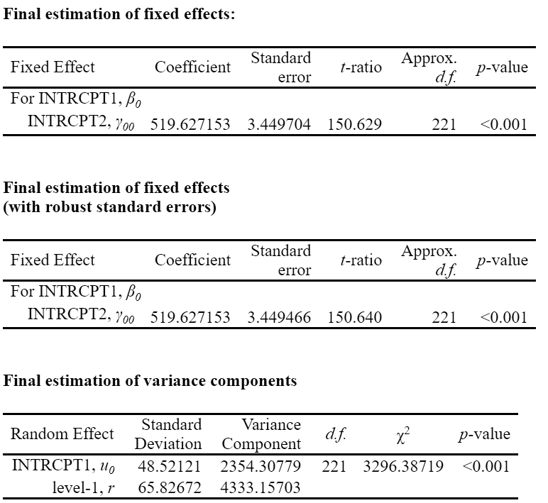
(Intercept) 519.627 3.449 150.654 3001.294 0.000 0.038 0.037
Estimate
Intercept~~Intercept|idschool 2354.330
Residual~~Residual 4331.574
ICC|idschool 0.352
Unadjusted hypothesis test as appropriate in larger samples.Comparing the results using HLM 8.0 shows similar results.
Note: An alternative way is to use the pool and the summary functions in the mice package. (Though the ICC cannot be computed based on this alone).
library(broom.mixed) #needed for summary to work?
mice::pool(mi_result2) %>% summary
## term estimate std.error statistic df p.value
## 1 (Intercept) 519.6271 3.44914 150.6541 1938.66 0The next regression includes both student- and school-level variables. [Just comparing the model-based standard errors and point estimates]
mi_result3 <- with(imp, lmer(math ~ sch_ses + parent_ed + likemath +
 (1|idschool),
REML = F, weight = nwt))
testEstimates(mi_result3, extra.pars = TRUE)
Call:

testEstimates(model = mi_result3, extra.pars = TRUE)

Final parameter estimates and inferences obtained from 5 imputed data sets.

             Estimate Std.Error   t.value        df   P(>|t|)       RIV       FMI
(Intercept)   452.198     4.555    99.277   892.770     0.000     0.072     0.069
sch_ses        21.144     2.536     8.338 23557.472     0.000     0.013     0.013
parent_ed       9.598     0.917    10.470   201.264     0.000     0.164     0.149
likemath       24.107     1.289    18.709   137.432     0.000     0.206     0.182

                              Estimate
Intercept~~Intercept|idschool 1450.405
Residual~~Residual            3949.023
ICC|idschool                     0.269

Unadjusted hypothesis test as appropriate in larger samples.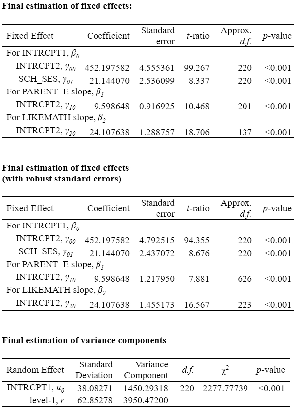
Single-level modeling can be used also accounting for the weights and clustering (using cluster robust standard errors using Taylor series linearization). Shown here is an example using the survey package. Note how the svydesign function is used and how the design object is used as the dataset.
library(survey)
des <- svydesign(ids = ~idschool, weights = ~nwt, data = imp)
s1 <- with(des, svyglm(math ~ sch_ses + parent_ed + likemath))
testEstimates(s1)
Call:
testEstimates(model = s1)
Final parameter estimates and inferences obtained from 5 imputed data sets.
Estimate Std.Error t.value df P(>|t|) RIV FMI
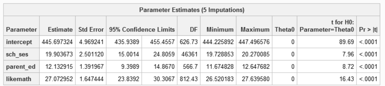
(Intercept) 445.697 4.968 89.713 626.126 0.000 0.087 0.083
sch_ses 19.904 2.500 7.960 46313.041 0.000 0.009 0.009
parent_ed 12.133 1.392 8.718 566.156 0.000 0.092 0.087
likemath 27.073 1.647 16.437 811.631 0.000 0.076 0.072
Unadjusted hypothesis test as appropriate in larger samples.If you compare the output with results using SAS surveyreg pooling the imputed results:
Extra: additional manual computations
NOTE: in the R object s1, this contains the results of the 5 regressions in a list format. If you want to see the results separately, can use:
lapply(s1, summary)$bsmmat01
Call:
svyglm(formula = math ~ sch_ses + parent_ed + likemath, design = .design)
Survey design:
svydesign(ids = ids, probs = probs, strata = strata, variables = variables,
fpc = fpc, nest = nest, check.strata = check.strata, weights = weights,
data = d, pps = pps, ...)
Coefficients:
Estimate Std. Error t value Pr(>|t|)
(Intercept) 445.861 4.732 94.216 < 2e-16 ***
sch_ses 19.852 2.533 7.837 2.01e-13 ***
parent_ed 11.977 1.323 9.054 < 2e-16 ***
likemath 27.013 1.582 17.078 < 2e-16 ***
---
Signif. codes: 0 '***' 0.001 '**' 0.01 '*' 0.05 '.' 0.1 ' ' 1
(Dispersion parameter for gaussian family taken to be 5288.907)
Number of Fisher Scoring iterations: 2
$bsmmat02
Call:
svyglm(formula = math ~ sch_ses + parent_ed + likemath, design = .design)
Survey design:
svydesign(ids = ids, probs = probs, strata = strata, variables = variables,
fpc = fpc, nest = nest, check.strata = check.strata, weights = weights,
data = d, pps = pps, ...)
Coefficients:
Estimate Std. Error t value Pr(>|t|)
(Intercept) 447.497 4.770 93.806 < 2e-16 ***
sch_ses 19.729 2.434 8.107 3.72e-14 ***
parent_ed 11.675 1.303 8.960 < 2e-16 ***
likemath 27.054 1.610 16.802 < 2e-16 ***
---
Signif. codes: 0 '***' 0.001 '**' 0.01 '*' 0.05 '.' 0.1 ' ' 1
(Dispersion parameter for gaussian family taken to be 5293.821)
Number of Fisher Scoring iterations: 2
$bsmmat03
Call:
svyglm(formula = math ~ sch_ses + parent_ed + likemath, design = .design)
Survey design:
svydesign(ids = ids, probs = probs, strata = strata, variables = variables,
fpc = fpc, nest = nest, check.strata = check.strata, weights = weights,
data = d, pps = pps, ...)
Coefficients:
Estimate Std. Error t value Pr(>|t|)
(Intercept) 446.168 4.771 93.511 < 2e-16 ***
sch_ses 20.270 2.509 8.080 4.39e-14 ***
parent_ed 12.044 1.349 8.927 < 2e-16 ***
likemath 27.640 1.561 17.704 < 2e-16 ***
---
Signif. codes: 0 '***' 0.001 '**' 0.01 '*' 0.05 '.' 0.1 ' ' 1
(Dispersion parameter for gaussian family taken to be 5354.77)
Number of Fisher Scoring iterations: 2
$bsmmat04
Call:
svyglm(formula = math ~ sch_ses + parent_ed + likemath, design = .design)
Survey design:
svydesign(ids = ids, probs = probs, strata = strata, variables = variables,
fpc = fpc, nest = nest, check.strata = check.strata, weights = weights,
data = d, pps = pps, ...)
Coefficients:
Estimate Std. Error t value Pr(>|t|)
(Intercept) 444.735 4.832 92.041 < 2e-16 ***
sch_ses 19.743 2.456 8.037 5.76e-14 ***
parent_ed 12.321 1.346 9.157 < 2e-16 ***
likemath 27.138 1.587 17.102 < 2e-16 ***
---
Signif. codes: 0 '***' 0.001 '**' 0.01 '*' 0.05 '.' 0.1 ' ' 1
(Dispersion parameter for gaussian family taken to be 5427.509)
Number of Fisher Scoring iterations: 2
$bsmmat05
Call:
svyglm(formula = math ~ sch_ses + parent_ed + likemath, design = .design)
Survey design:
svydesign(ids = ids, probs = probs, strata = strata, variables = variables,
fpc = fpc, nest = nest, check.strata = check.strata, weights = weights,
data = d, pps = pps, ...)
Coefficients:
Estimate Std. Error t value Pr(>|t|)
(Intercept) 444.226 4.720 94.115 < 2e-16 ***
sch_ses 19.924 2.511 7.935 1.1e-13 ***
parent_ed 12.648 1.338 9.452 < 2e-16 ***
likemath 26.520 1.600 16.571 < 2e-16 ***
---
Signif. codes: 0 '***' 0.001 '**' 0.01 '*' 0.05 '.' 0.1 ' ' 1
(Dispersion parameter for gaussian family taken to be 5438.649)
Number of Fisher Scoring iterations: 2The results are slightly different for each regression (since the outcome changes slightly for each because of the PVs).
To see the results only for one variable (sch_ses as an example):
#lapply(s1, function(x) summary(x)$coef[2,])
tmp <- lapply(s1, function(x) summary(x)$coef[2,])
(sch_ses <- data.frame(do.call(rbind, tmp)))
Estimate Std..Error t.value Pr...t..
bsmmat01 19.85218 2.533036 7.837306 2.011657e-13
bsmmat02 19.72885 2.433623 8.106783 3.717540e-14
bsmmat03 20.27009 2.508550 8.080401 4.391472e-14
bsmmat04 19.74307 2.456446 8.037250 5.763590e-14
bsmmat05 19.92418 2.511053 7.934591 1.097265e-13The regression coefficient is just the average of the estimates:
mean(sch_ses$Estimate)## [1] 19.90367The total variance (denoted by \(T\)) of the coefficient is:
\[T = \bar{U} + (1 + \frac{1}{m}) \times B\]
- U = mean of the variance of the coefficients (square the standard errors)
- B = variance of the regression coefficients
- m = number of imputations
Ubar <- mean(sch_ses$Std..Error^2)
B <- var(sch_ses$Estimate)
adj <- (1 + (1/5))
Putting it all together (the second part of the equation is an adjustment which increases the variability):
(Ubar + adj * B) #that's the variance## [1] 6.252331sqrt(Ubar + adj * B) #this is the standard error## [1] 2.500466Compare this with the combined imputed results (i.e., B = 1.90, SE = 2.50).
Getting descriptives using complex imputed survey data
Now a basic task is to, of course, present descriptives of the imputed data (i.e., Means and SDs). Running the regression was easy. This took me a longer time to figure out. [reminder: we don’t really have imputed data here but it will work the same way.]
You can use the svymean function in the survey package. And then combine them using the miceadds::withPool_MI() in the miceadds package (yes, another package to install). The MIcombine in the mitools package would also work though this does not work with the svyvar function (there is no svysd function: but that function can be found in yet another package, jtools).
For now, let us just stick wit the withPool_MI function as that works for everything we need.
# with(des, svymean(~math + parent_ed + sch_ses + books)) %>% MIcombine
# the above will work but will not work with variances so be warned

with(des, svymean(~math + parent_ed + sch_ses + books)) %>% miceadds::withPool_MI()
mean SE
math 523.9700 3.4650
parent_ed 3.0664 0.0379
sch_ses 1.0816 0.0768
books 2.0031 0.0420We can save this in an object and extract the data so we do not have to manually type these in:
ms <- with(des, svymean(~math + parent_ed + sch_ses + books)) %>% miceadds::withPool_MI()
ms[1:4] #these are the means of the first four variables
math parent_ed sch_ses books
523.969966 3.066350 1.081585 2.003147 ## NOTE, only math actually needed this, the other variables
## are all completely observed so will not varySome variables are completely observed (no missing), so will be the same as:
dat1 <- imp$imputations$bsmmat01 #first dataset
weighted.mean(dat1$parent_ed, dat1$totwgt)
[1] 3.06635You could get the SDs by using the svyvar function and taking the square root (sqrt). This is just not labeled properly as its says variance and not SD so be warned (know what you are doing, do not just blindly follow this). The MIcombine function does not work with multiple variables which is why we are using the function in miceadds instead
with(des, svyvar(~math + parent_ed + sch_ses + books)) %>%
  miceadds::withPool_MI() %>%
  sqrt
variance SE
math 81.5820 268.9323
parent_ed 1.1174 0.0381
sch_ses 1.0868 0.0877
books 1.2990 0.0295You can save this into an object as well:
sds <- with(des, svyvar(~math + parent_ed + sch_ses + books)) %>%
  miceadds::withPool_MI()
sds #these are variances
variance SE
math 6655.6170 268.9323
parent_ed 1.2485 0.0381
sch_ses 1.1812 0.0877
books 1.6875 0.0295diag(sqrt(sds)) #need to do this because it is a math parent_ed sch_ses books
81.581965 1.117351 1.086833 1.299022 #variance covariance matrix. The variances are on the
#diagonals so need to get the square root to get
#SDsPutting all together in a descriptive table (which you can easily export):
data.frame(M = ms[1:4], SD = diag(sqrt(sds))) M SD
math 523.969966 81.581965
parent_ed 3.066350 1.117351
sch_ses 1.081585 1.086833
books 2.003147 1.299022Seems like a lot of work to get the descriptives.
If you want the counts of the categorical variables… have to do this one at a time. The numbers are not integers since they are weighted.
#with(des, svytable(~books)) %>% MIcombine #will not work
with(des, svytable(~books)) %>% miceadds::withPool_MI()
books
0 1 2 3 4
868.7026 1196.4360 1657.9400 978.0992 986.8221 – end