Multilevel CFA (MLCFA) in R, part 2
A while back, I wrote a note about how to conduct a multilevel
confirmatory factor analysis (MLCFA) in
R. Part of the
note shows how to setup lavaan to be able to run the MLCFA model.
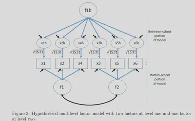
NOTE: one of the important aspects of an MLCFA is that the factor
structure at the two levels may not be the same– that is the factor
structures are invariant across levels. The setup process is/was
cumbersome– but putting the note together was informative. Testing a 2-1
factor model (i.e., 2 factors at the first level and 1 factor at the
second level) required the following code (see the original note for the
detailed explanation of the setup and what the variables represent).
This is a measure of school engagement; n = 3,894 students in 254
schools.
1. Running an MLCFA manually
- Read in the data
library(lavaan)
source("https://raw.githubusercontent.com/flh3/mcfa/main/02_syntax/mcfa2.R")
raw <- read.csv("https://raw.githubusercontent.com/flh3/mcfa/main/01_data/raw.csv")
head(raw)

  x1 x2 x3 x4 x5 x6 sid
1  4  4  3  4  4  3  55
2  6  6  4  6  4  4  55
3  5  5  2  6  4  4  55
4  4  4  5  5  3  3  55
5  4  4  4  4  3  2  55
6  4  4  2  4  2  2  55
Just as a reminder, here are some item statistics: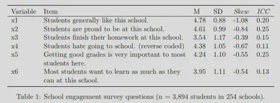
- Prepare the data for use with the
mcfa.inputfunction to create the necessary matrices and store them inx.
x <- mcfa.input("sid", raw) #sid is the school id or clustering variable
combined.cov <- list(within = x$pw.cov, between = x$b.cov)
combined.n <- list(within = x$n - x$G, between = x$G)
x$icc #view intraclass correlation (ICCs) of the six variables

   x1    x2    x3    x4    x5    x6
0.199 0.247 0.145 0.108 0.248 0.125
- Specify the model:
level2.1factor <- '
  f1 =~ x1 + c(a,a)*x2 + c(b,b)*x4
  f2 =~ x3 + c(c,c)*x5 + c(d,d)*x6

  x1 ~~ c(e,e)*x1
  x2 ~~ c(f,f)*x2
  x3 ~~ c(g,g)*x3
  x4 ~~ c(h,h)*x4
  x5 ~~ c(i,i)*x5
  x6 ~~ c(j,j)*x6
  f1 ~~ c(k,k)*f1
  f2 ~~ c(l,l)*f2
  f1 ~~ c(m,m)*f2
  x1b =~ c(0,3.91)*x1
  x1b ~~ c(0,NA)*x1b
  x2b =~ c(0,3.91)*x2
  x2b ~~ c(0,NA)*x2b
  x3b =~ c(0,3.91)*x3
  x3b ~~ c(0,NA)*x3b
  x4b =~ c(0,3.91)*x4
  x4b ~~ c(0,NA)*x4b
  x5b =~ c(0,3.91)*x5
  x5b ~~ c(0,NA)*x5b
  x6b =~ c(0,3.91)*x6
  x6b ~~ c(0,NA)*x6b

  bf1 =~ c(0,1)*x1b  + c(0,NA)*x2b + c(0,NA)*x3b + c(0,NA)*x4b  +
     c(0,NA)*x5b + c(0,NA)*x6b
  bf1 ~~ c(0,NA)*bf1 + c(0,0)*f1 + c(0,0)*f2
'
The specified model looks like:
- Run the model:
results6 <- cfa(level2.1factor, sample.cov = combined.cov,
 sample.nobs = combined.n, orthogonal = T)
summary(results6, fit.measures = T, standardized = T)

lavaan 0.6-19 ended normally after 54 iterations

  Estimator                                         ML
  Optimization method                           NLMINB
  Number of model parameters                        38
  Number of equality constraints                    13

  Number of observations per group:
    within                                        3640
    between                                        254

Model Test User Model:

  Test statistic                               142.465
  Degrees of freedom                                17
  P-value (Chi-square)                           0.000
  Test statistic for each group:
    within                                      56.924
    between                                     85.541

Model Test Baseline Model:

  Test statistic                             11054.075
  Degrees of freedom                                30
  P-value                                        0.000

User Model versus Baseline Model:

  Comparative Fit Index (CFI)                    0.989
  Tucker-Lewis Index (TLI)                       0.980

Loglikelihood and Information Criteria:

  Loglikelihood user model (H0)             -27509.959
  Loglikelihood unrestricted model (H1)     -27438.727

  Akaike (AIC)                               55069.919
  Bayesian (BIC)                             55226.599
  Sample-size adjusted Bayesian (SABIC)      55147.160

Root Mean Square Error of Approximation:

  RMSEA                                          0.062
  90 Percent confidence interval - lower         0.052
  90 Percent confidence interval - upper         0.071
  P-value H_0: RMSEA <= 0.050                    0.019
  P-value H_0: RMSEA >= 0.080                    0.001

Standardized Root Mean Square Residual:

  SRMR                                           0.024

Parameter Estimates:

  Standard errors                             Standard
  Information                                 Expected
  Information saturated (h1) model          Structured


Group 1 [within]:

Latent Variables:
                   Estimate  Std.Err  z-value  P(>|z|)   Std.lv  Std.all
  f1 =~
    x1                1.000                               0.694    0.882
    x2         (a)    1.081    0.021   51.609    0.000    0.750    0.873
    x4         (b)    0.649    0.024   27.156    0.000    0.450    0.454
  f2 =~
    x3                1.000                               0.688    0.634
    x5         (c)    1.146    0.030   38.404    0.000    0.789    0.819
    x6         (d)    1.317    0.034   38.786    0.000    0.906    0.868
  x1b =~
    x1                0.000                               0.000    0.000
  x2b =~
    x2                0.000                               0.000    0.000
  x3b =~
    x3                0.000                               0.000    0.000
  x4b =~
    x4                0.000                               0.000    0.000
  x5b =~
    x5                0.000                               0.000    0.000
  x6b =~
    x6                0.000                               0.000    0.000
  bf1 =~
    x1b               0.000                                 NaN      NaN
    x2b               0.000                                 NaN      NaN
    x3b               0.000                                 NaN      NaN
    x4b               0.000                                 NaN      NaN
    x5b               0.000                                 NaN      NaN
    x6b               0.000                                 NaN      NaN

Covariances:
                   Estimate  Std.Err  z-value  P(>|z|)   Std.lv  Std.all
  f1 ~~
    f2         (m)    0.301    0.013   24.014    0.000    0.630    0.630
    bf1               0.000                                 NaN      NaN
  f2 ~~
    bf1               0.000                                 NaN      NaN

Variances:
                   Estimate  Std.Err  z-value  P(>|z|)   Std.lv  Std.all
   .x1         (e)    0.137    0.008   17.000    0.000    0.137    0.222
   .x2         (f)    0.176    0.010   18.328    0.000    0.176    0.238
   .x3         (g)    0.704    0.019   37.860    0.000    0.704    0.598
   .x4         (h)    0.781    0.019   41.160    0.000    0.781    0.794
   .x5         (i)    0.306    0.012   25.779    0.000    0.306    0.330
   .x6         (j)    0.270    0.014   19.493    0.000    0.270    0.247
    f1         (k)    0.481    0.016   30.196    0.000    1.000    1.000
    f2         (l)    0.473    0.024   20.059    0.000    1.000    1.000
   .x1b               0.000                                 NaN      NaN
   .x2b               0.000                                 NaN      NaN
   .x3b               0.000                                 NaN      NaN
   .x4b               0.000                                 NaN      NaN
   .x5b               0.000                                 NaN      NaN
   .x6b               0.000                                 NaN      NaN
    bf1               0.000                                 NaN      NaN


Group 2 [between]:

Latent Variables:
                   Estimate  Std.Err  z-value  P(>|z|)   Std.lv  Std.all
  f1 =~
    x1                1.000                               0.694    0.407
    x2         (a)    1.081    0.021   51.609    0.000    0.750    0.360
    x4         (b)    0.649    0.024   27.156    0.000    0.450    0.270
  f2 =~
    x3                1.000                               0.688    0.343
    x5         (c)    1.146    0.030   38.404    0.000    0.789    0.345
    x6         (d)    1.317    0.034   38.786    0.000    0.906    0.496
  x1b =~
    x1                3.910                               1.511    0.887
  x2b =~
    x2                3.910                               1.900    0.911
  x3b =~
    x3                3.910                               1.685    0.841
  x4b =~
    x4                3.910                               1.341    0.804
  x5b =~
    x5                3.910                               2.073    0.907
  x6b =~
    x6                3.910                               1.497    0.820
  bf1 =~
    x1b               1.000                               0.987    0.987
    x2b               1.258    0.037   33.807    0.000    0.987    0.987
    x3b               1.025    0.062   16.612    0.000    0.906    0.906
    x4b               0.784    0.054   14.640    0.000    0.871    0.871
    x5b               1.256    0.064   19.471    0.000    0.903    0.903
    x6b               0.991    0.047   21.132    0.000    0.986    0.986

Covariances:
                   Estimate  Std.Err  z-value  P(>|z|)   Std.lv  Std.all
  f1 ~~
    f2         (m)    0.301    0.013   24.014    0.000    0.630    0.630
    bf1               0.000                               0.000    0.000
  f2 ~~
    bf1               0.000                               0.000    0.000

Variances:
                   Estimate  Std.Err  z-value  P(>|z|)   Std.lv  Std.all
   .x1         (e)    0.137    0.008   17.000    0.000    0.137    0.047
   .x2         (f)    0.176    0.010   18.328    0.000    0.176    0.040
   .x3         (g)    0.704    0.019   37.860    0.000    0.704    0.175
   .x4         (h)    0.781    0.019   41.160    0.000    0.781    0.281
   .x5         (i)    0.306    0.012   25.779    0.000    0.306    0.058
   .x6         (j)    0.270    0.014   19.493    0.000    0.270    0.081
    f1         (k)    0.481    0.016   30.196    0.000    1.000    1.000
    f2         (l)    0.473    0.024   20.059    0.000    1.000    1.000
   .x1b               0.004    0.002    1.742    0.082    0.027    0.027
   .x2b               0.006    0.003    1.812    0.070    0.025    0.025
   .x3b               0.033    0.008    4.161    0.000    0.179    0.179
   .x4b               0.028    0.007    3.814    0.000    0.241    0.241
   .x5b               0.052    0.008    6.639    0.000    0.185    0.185
   .x6b               0.004    0.004    0.985    0.325    0.027    0.027
    bf1               0.145    0.017    8.637    0.000    1.000    1.000
2. Automatic Setup of an MLCFA
To run this automatically using lavaan, the setup is now much
simpler:
twolevel <- '
level: 1
  f1 =~ x1 + x2 + x4
  f2 =~ x3 + x5 + x6
level: 2
  fb =~ x1 + x2 + x3 + x4 + x5 + x6
'

results <- cfa(twolevel, data = raw, cluster = 'sid')

Warning: lavaan->lav_data_full():
   Level-1 variable "x1" has no variance within some clusters . The cluster ids with zero within variance are: 62, 52, 54.

Warning: lavaan->lav_data_full():
   Level-1 variable "x2" has no variance within some clusters . The cluster ids with zero within variance are: 61.

Warning: lavaan->lav_data_full():
   Level-1 variable "x5" has no variance within some clusters . The cluster ids with zero within variance are: 60.

summary(results, fit.measures = T, standardized = T)

lavaan 0.6-19 ended normally after 73 iterations

  Estimator                                         ML
  Optimization method                           NLMINB
  Number of model parameters                        31

  Number of observations                          3894
  Number of clusters [sid]                         254

Model Test User Model:

  Test statistic                               140.120
  Degrees of freedom                                17
  P-value (Chi-square)                           0.000

Model Test Baseline Model:

  Test statistic                             10988.837
  Degrees of freedom                                30
  P-value                                        0.000

User Model versus Baseline Model:

  Comparative Fit Index (CFI)                    0.989
  Tucker-Lewis Index (TLI)                       0.980

Loglikelihood and Information Criteria:

  Loglikelihood user model (H0)             -27492.948
  Loglikelihood unrestricted model (H1)     -27422.888

  Akaike (AIC)                               55047.896
  Bayesian (BIC)                             55242.179
  Sample-size adjusted Bayesian (SABIC)      55143.675

Root Mean Square Error of Approximation:

  RMSEA                                          0.043
  90 Percent confidence interval - lower         0.037
  90 Percent confidence interval - upper         0.050
  P-value H_0: RMSEA <= 0.050                    0.953
  P-value H_0: RMSEA >= 0.080                    0.000

Standardized Root Mean Square Residual (corr metric):

  SRMR (within covariance matrix)                0.022
  SRMR (between covariance matrix)               0.055

Parameter Estimates:

  Standard errors                             Standard
  Information                                 Observed
  Observed information based on                Hessian


Level 1 [within]:

Latent Variables:
                   Estimate  Std.Err  z-value  P(>|z|)   Std.lv  Std.all
  f1 =~
    x1                1.000                               0.693    0.881
    x2                1.084    0.021   52.810    0.000    0.751    0.874
    x4                0.644    0.024   27.003    0.000    0.446    0.449
  f2 =~
    x3                1.000                               0.688    0.634
    x5                1.146    0.030   38.464    0.000    0.789    0.819
    x6                1.321    0.034   38.847    0.000    0.908    0.869

Covariances:
                   Estimate  Std.Err  z-value  P(>|z|)   Std.lv  Std.all
  f1 ~~
    f2                0.301    0.012   24.171    0.000    0.631    0.631

Variances:
                   Estimate  Std.Err  z-value  P(>|z|)   Std.lv  Std.all
   .x1                0.138    0.008   17.530    0.000    0.138    0.223
   .x2                0.175    0.009   18.669    0.000    0.175    0.237
   .x4                0.790    0.019   41.008    0.000    0.790    0.799
   .x3                0.705    0.019   38.015    0.000    0.705    0.598
   .x5                0.306    0.012   25.811    0.000    0.306    0.329
   .x6                0.269    0.014   19.432    0.000    0.269    0.246
    f1                0.481    0.016   30.197    0.000    1.000    1.000
    f2                0.473    0.024   19.969    0.000    1.000    1.000


Level 2 [sid]:

Latent Variables:
                   Estimate  Std.Err  z-value  P(>|z|)   Std.lv  Std.all
  fb =~
    x1                1.000                               0.385    0.988
    x2                1.262    0.037   34.134    0.000    0.486    0.986
    x3                0.997    0.067   14.861    0.000    0.384    0.899
    x4                0.790    0.054   14.611    0.000    0.304    0.911
    x5                1.209    0.071   17.078    0.000    0.466    0.898
    x6                0.987    0.050   19.704    0.000    0.380    0.988

Intercepts:
                   Estimate  Std.Err  z-value  P(>|z|)   Std.lv  Std.all
   .x1                4.744    0.028  168.611    0.000    4.744   12.167
   .x2                4.564    0.035  131.910    0.000    4.564    9.253
   .x3                3.513    0.033  107.212    0.000    3.513    8.225
   .x4                4.348    0.027  160.857    0.000    4.348   13.024
   .x5                4.198    0.037  114.219    0.000    4.198    8.095
   .x6                3.913    0.030  130.439    0.000    3.913   10.168

Variances:
                   Estimate  Std.Err  z-value  P(>|z|)   Std.lv  Std.all
   .x1                0.004    0.002    1.824    0.068    0.004    0.024
   .x2                0.007    0.003    2.271    0.023    0.007    0.028
   .x3                0.035    0.008    4.100    0.000    0.035    0.191
   .x4                0.019    0.008    2.495    0.013    0.019    0.170
   .x5                0.052    0.008    6.554    0.000    0.052    0.193
   .x6                0.003    0.004    0.946    0.344    0.003    0.023
    fb                0.148    0.018    8.274    0.000    1.000    1.000
The factor loadings and fit indices are similar– and are exactly the
same when done using Mplus (see article p. 15 for a comparison).
To get the alpha at either level (part of the function), can use the
alpha function (I prefer Omega nowadays though for several reasons).
alpha(x$ab.cov) #multilevel alpha or level 2 alpha

[1] 0.9658581
NOTE: At the moment, you cannot use ordinal data in a two level model
using lavaan and WLSMV.
- END