Correct standard errors?

The other day in class, while talking about instances (e.g., analyzing clustered data or heteroskedastic residuals) where adjustments are required to the standard errors of a regression model, a student asked: how do we know what the ‘true’ standard error should be in the first place– which is necessary to know if it is too high or too low.

This short simulation illustrates that, over repeated sampling from a specified population, the standard deviaton of the regression coefficients can be used as the true standard errors. Take for example the case where the residuals of a regression are heteroskedastic instead of the assumed homoskedastic residuals. Parameter estimates will be unbiased but the standard errors will be biased.

To illustrate this, I create one dataset which shows heteroskedastic residuals:

set.seed(2468)
ns <- 400 #sample size
B1 <- 3 #regression coefficient
x1 <- runif(ns, 10, 30)
err <- rnorm(ns, 0, x1^2) #variance [or sd] increases as x1 increases
y <- 50 + B1 * x1 + err

m1 <- lm(y ~ x1) #run a basic regression
summary(m1) #we see that the the coefficient for x1

## 
## Call:
## lm(formula = y ~ x1)
## 
## Residuals:
##      Min       1Q   Median       3Q      Max 
## -1980.99  -274.52     7.57   270.21  1458.05 
## 
## Coefficients:
##             Estimate Std. Error t value Pr(>|t|)
## (Intercept)   40.230     95.180   0.423    0.673
## x1             2.907      4.667   0.623    0.534
## 
## Residual standard error: 506.3 on 398 degrees of freedom
## Multiple R-squared:  0.000974,   Adjusted R-squared:  -0.001536 
## F-statistic: 0.388 on 1 and 398 DF,  p-value: 0.5337

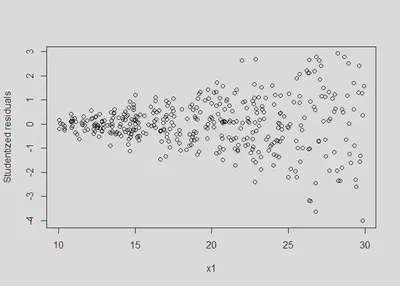
plot(x1, rstudent(m1), ylab = 'Studentized residuals') #classic fan spread of residuals

library(lmtest)

bptest(m1) #Breusch Pagan test: results show statistical significance indicating a violation

## 
##  studentized Breusch-Pagan test
## 
## data:  m1
## BP = 98.226, df = 1, p-value < 2.2e-16

However, the question then becomes: what should the standard error be? So, we can run a simulation where we run a regression 1,000 times (1,000 replications) and collect the output. Typically, using heteroskedasticity corrected standard errors should alleviate the problem which we will see.

set.seed(123)
ns <- 400 #sample size
B1 <- 3 #regression coefficient
reps <- 500 #replications

#container to save the coefficient and the standard errors
cfs <- ses <- ses2 <- matrix(NA, ncol = 2, nrow = reps)

library(sandwich) #to get the adjusted standard errors

set.seed(3210) #for reproducability
#the actual simulation
for (i in 1:reps){
  x1 <- runif(ns, 10, 30)
  err <- rnorm(ns, 0, x1^2) #variance [or sd] increases as x1 increases
  y <- 50 + B1 * x1 + err
  m2 <- lm(y ~ x1) #run a basic regression
  cfs[i, ] <- coef(m2)
  ses[i, ] <- sqrt(diag(vcov(m2)))
  ses2[i, ] <- sqrt(diag(vcovHC(m2) ))
  #cat(i, "::")
}

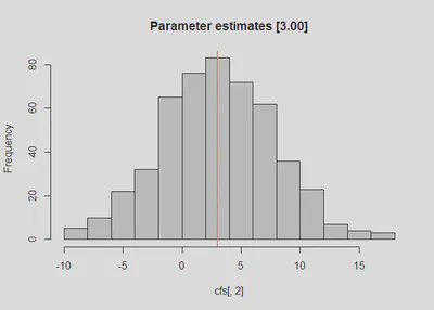
After running the simulation, we can compare the actual standard errors to the empirically determined standard errors. The point estimate is ~ 3.00 (i.e., \(B = 3.04\)).

### these are for the point estimates: should be unbiased
colMeans(cfs) #should be around 50 and 3.00

## [1] 47.974758  3.044893

hist(cfs[,2], main = 'Parameter estimates [3.00]')
abline(v = 3, col = 'red')

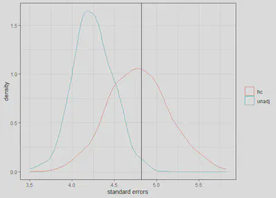
For the standard errors, we can compare the 1) empirical standard errors; 2) the unadjusted standard errors; and 3) the corrected standard errors.

### these are for the standard errors
apply(cfs, 2, sd) #these show the empirical standard errors for the intercept and x1

## [1] 78.909899  4.819149

colMeans(ses) #these are the model based standard errors

## [1] 88.474339  4.247855

colMeans(ses2) #these are adjusted standard errors

## [1] 78.28279  4.78608

We can see that the unadjusted standard errors for \(x_{1}\) are too low ((4.24 - 4.82)/4.82 = -12%) while the adjusted standard errors are close to the empirical standard errors (i.e., 4.79 vs. 4.82).

dat <- data.frame(se = c(ses[,2], ses2[,2]), gr = rep(c('unadj', 'hc'), each = reps))

library(ggplot2)
ggplot(dat, aes(x = se, group = gr, col = factor(gr))) +
 geom_density() +
 geom_vline(xintercept = sd(cfs[,2])) + 
  theme_bw() +
  labs(col = "", x = 'standard errors')