(MLM notes). Residuals are often used for model diagnostics or for spotting outliers in the data. For single-level models, these are merely the observed - predicted data (i.e., \(y_i - \hat{y}_i\)). However, for multilevel models, these are a bit more complicated to compute. Since we have two error terms (in this example), we will have two sets of residuals. For example, a multilevel model with a single predictor at level one can be written as:
\[y_{ij} = \gamma_{00} + \gamma_{01}x_{ij} + u_{0j} + r_{ij}\] The \(u_{0j}\) represent the estimated level-2 residuals and are assumed to be normally distributed with a mean of 0 and variance of \(\tau_{00}\) or \(\mathcal{N}\sim(0, \tau_{00})\).
Read in and examine the data
A small three cluster dataset (comb) is used (so we can see and compare results of our computations done manually and automatically using functions). There are only 20 observations in the data nested within 3 clusters.
library(lme4)
library(MLMusingR)
library(ggplot2)

load(url("https://github.com/flh3/pubdata/raw/main/miscdata/three_groups.rda"))
comb <- three_group
names(comb)[2] <- "xij" #just renaming
ggplot(comb, aes(x = xij, y = y, group = gp, col = gp)) +
  geom_point() +
  geom_smooth(method = 'lm', se = F) + theme_bw() +
  labs(col = '')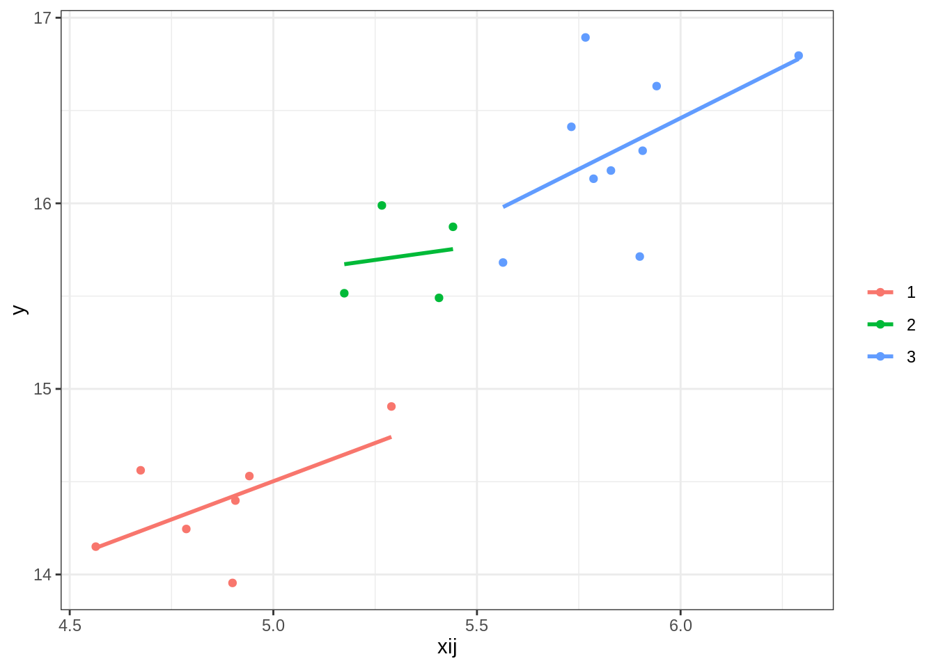
Fit a random intercept model
m1 <- lmer(y ~ xij + (1|gp), data = comb)
summary(m1)
Linear mixed model fit by REML ['lmerMod']
Formula: y ~ xij + (1 | gp)
Data: comb
REML criterion at convergence: 18.9
Scaled residuals:
Min 1Q Median 3Q Max
-1.91641 -0.25110 -0.01964 0.36049 2.17381
Random effects:
Groups Name Variance Std.Dev.
gp (Intercept) 0.2142 0.4628
Residual 0.1066 0.3266
Number of obs: 20, groups: gp, 3
Fixed effects:
Estimate Std. Error t value
(Intercept) 9.2389 1.8492 4.996
xij 1.1645 0.3416 3.409
Correlation of Fixed Effects:
(Intr)
xij -0.989We will use the m1 object in our computations. We can first begin by extracting our variance components of \(\tau_{00}\) and \(\sigma^2\) from the merMod object.
# extract and save variance components
T00 <- data.frame(VarCorr(m1))$vcov[1]
sig2 <- sigma(m1)^2
We also of course still need to get the predicted values. With MLMs, you can get the conditional predicted values (that include the random effects) and the marginal predicted values (only using the fixed effects). For this, we need the marginal values. We can compute this using some basic matrix algebra and compare it to the predicted values using the predict function (note the re.form = NA option).
X <- model.matrix(m1) # the design matrix
B <- fixef(m1) # the regression coefficients
(comb$yhat <- as.numeric(X %*% B))
[1] 14.94475 14.68207 14.55376 14.99295 14.95298 15.39909 14.81260 15.26433
[9] 15.37181 15.57521 15.53524 16.10927 15.95407 15.71827 15.91369 16.15747
[17] 16.11750 16.56360 15.97712 16.02679predict(m1, re.form = NA) # the same 1 2 4 6 7 8 9 12
14.94475 14.68207 14.55376 14.99295 14.95298 15.39909 14.81260 15.26433
13 16 17 21 23 24 25 26
15.37181 15.57521 15.53524 16.10927 15.95407 15.71827 15.91369 16.15747
27 28 29 30
16.11750 16.56360 15.97712 16.02679 From here, we can compute the residuals as in the single-level model (\(y_{ij} - \hat{y}_{ij}\)). We will use these in our computations of our level-specific residuals.
# computing raw residuals (obs - predicted)
comb$resid <- comb$y - comb$yhat
We also need the average residuals per group. These estimates will then be shrunken using a shrinkage factor (or the reliability). The depends on the random effect estimates and the number of observations within each cluster j. If the sample sizes were balanced, this would be the same for each cluster. The more observations in a cluster, the more reliable the estimate.
# computing average raw residuals per group
comb$rj <- group_mean(comb$resid, comb$gp) #function is from MLMusingR
The shrinkage factor uses the reliability of the random effects (i.e., the intercept) per group (\(\frac{\tau_{00}}{\tau_{00} + \sigma^2/n_j}\)).
# how many in each cluster
(nj <- table(comb$gp))
1 2 3
7 4 9
# computing shrinkage factor
shrink <- T00 / (T00 + sig2/ nj)
names(shrink) <- names(nj)
tmp <- data.frame(shrink)
names(tmp) <- c('gp', 'shrink')
tmp gp shrink
1 1 0.9335809
2 2 0.8892819
3 3 0.9475668# merging shrinkage estimates to the dataset
comb <- merge(comb, tmp, by = 'gp')The shrunken random effects are the average random effect per group (rj) \(\times\) the shrinkage factor (or the reliability of the residuals). These residuals are referred to as precision weighted.
comb$rj2 <- comb$rj * comb$shrink # shrunken
comb$rj2[!duplicated(comb$rj2)]
[1] -0.4791212 0.2493284 0.2297928ranef(m1) # same as this if using a function$gp
(Intercept)
1 -0.4791212
2 0.2493284
3 0.2297928
with conditional variances for "gp" Now we can compute the residuals at level one as the residuals - the random effects associated with the cluster.
comb$residm <- as.numeric(comb$resid - comb$rj2) # computed manually
comb$residauto <- as.numeric(resid(m1)) # extracted using a function
all.equal(comb$residm, comb$residauto)
[1] TRUEcomb gp y xij yhat resid rj shrink rj2
1 1 13.95463 4.899748 14.94475 -0.99012325 -0.5132080 0.9335809 -0.4791212
2 1 14.56151 4.674181 14.68207 -0.12056692 -0.5132080 0.9335809 -0.4791212
3 1 14.15016 4.563992 14.55376 -0.40359832 -0.5132080 0.9335809 -0.4791212
4 1 14.53039 4.941141 14.99295 -0.46255936 -0.5132080 0.9335809 -0.4791212
5 1 14.39840 4.906820 14.95298 -0.55458876 -0.5132080 0.9335809 -0.4791212
6 1 14.90533 5.289899 15.39909 -0.49375817 -0.5132080 0.9335809 -0.4791212
7 1 14.24534 4.786271 14.81260 -0.56726099 -0.5132080 0.9335809 -0.4791212
8 2 15.51547 5.174181 15.26433 0.25113911 0.2803705 0.8892819 0.2493284
9 2 15.98862 5.266476 15.37181 0.61681157 0.2803705 0.8892819 0.2493284
10 2 15.87341 5.441141 15.57521 0.29819517 0.2803705 0.8892819 0.2493284
11 2 15.49058 5.406820 15.53524 -0.04466399 0.2803705 0.8892819 0.2493284
12 3 15.71321 5.899748 16.10927 -0.39605333 0.2425083 0.9475668 0.2297928
13 3 16.89377 5.766476 15.95407 0.93969967 0.2425083 0.9475668 0.2297928
14 3 15.68102 5.563992 15.71827 -0.03725480 0.2425083 0.9475668 0.2297928
15 3 16.41222 5.731801 15.91369 0.49853464 0.2425083 0.9475668 0.2297928
16 3 16.63160 5.941141 16.15747 0.47413488 0.2425083 0.9475668 0.2297928
17 3 16.28345 5.906820 16.11750 0.16594631 0.2425083 0.9475668 0.2297928
18 3 16.79600 6.289899 16.56360 0.23239852 0.2425083 0.9475668 0.2297928
19 3 16.13245 5.786271 15.97712 0.15533167 0.2425083 0.9475668 0.2297928
20 3 16.17663 5.828927 16.02679 0.14983670 0.2425083 0.9475668 0.2297928
residm residauto
1 -0.511002081 -0.511002081
2 0.358554242 0.358554242
3 0.075522843 0.075522843
4 0.016561807 0.016561807
5 -0.075467600 -0.075467600
6 -0.014637005 -0.014637005
7 -0.088139826 -0.088139826
8 0.001810718 0.001810718
9 0.367483175 0.367483175
10 0.048866779 0.048866779
11 -0.293992384 -0.293992384
12 -0.625846103 -0.625846103
13 0.709906902 0.709906902
14 -0.267047570 -0.267047570
15 0.268741869 0.268741869
16 0.244342114 0.244342114
17 -0.063846463 -0.063846463
18 0.002605752 0.002605752
19 -0.074461098 -0.074461098
20 -0.079956070 -0.079956070Side note: computing conditional predicted values
The conditional predicted value is \(\hat{y}_{ij} = XB + Zu\).
z <- matrix(getME(m1, 'Z'), ncol = 3) # random effect design matrix
u <- ranef(m1)[[1]]$'(Intercept)' # random effects shrunken

# getting predicted values (manually)
as.numeric(X %*% B + z %*% u) # manual
[1] 14.46563 14.20295 14.07463 14.51383 14.47386 14.91997 14.33348 15.51366
[9] 15.62114 15.82454 15.78457 16.33906 16.18386 15.94806 16.14348 16.38726
[17] 16.34729 16.79340 16.20691 16.25659Can compare this using the function fitted or predict:
fitted(m1) # or predict(m1) (using a function) 1 2 4 6 7 8 9 12
14.46563 14.20295 14.07463 14.51383 14.47386 14.91997 14.33348 15.51366
13 16 17 21 23 24 25 26
15.62114 15.82454 15.78457 16.33906 16.18386 15.94806 16.14348 16.38726
27 28 29 30
16.34729 16.79340 16.20691 16.25659 comb$y - comb$residm # obs - residual [1] 14.46563 14.20295 14.07463 14.51383 14.47386 14.91997 14.33348 15.51366
[9] 15.62114 15.82454 15.78457 16.33906 16.18386 15.94806 16.14348 16.38726
[17] 16.34729 16.79340 16.20691 16.25659# plotting per group
ggplot(comb, aes(x = xij, y = fitted(m1))) +
geom_point(aes(x = xij, y = y)) + #observed
#geom_smooth(method = 'lm', se = F, lty = 'dashed', alpha = .5, width = .5) + # overall
geom_smooth(aes(x = xij, y = fitted(m1), col = factor(gp))) + # per cluster
labs(col = '', y = 'y') +
geom_abline(intercept = fixef(m1)[1], slope = fixef(m1)[2]) +
theme_bw()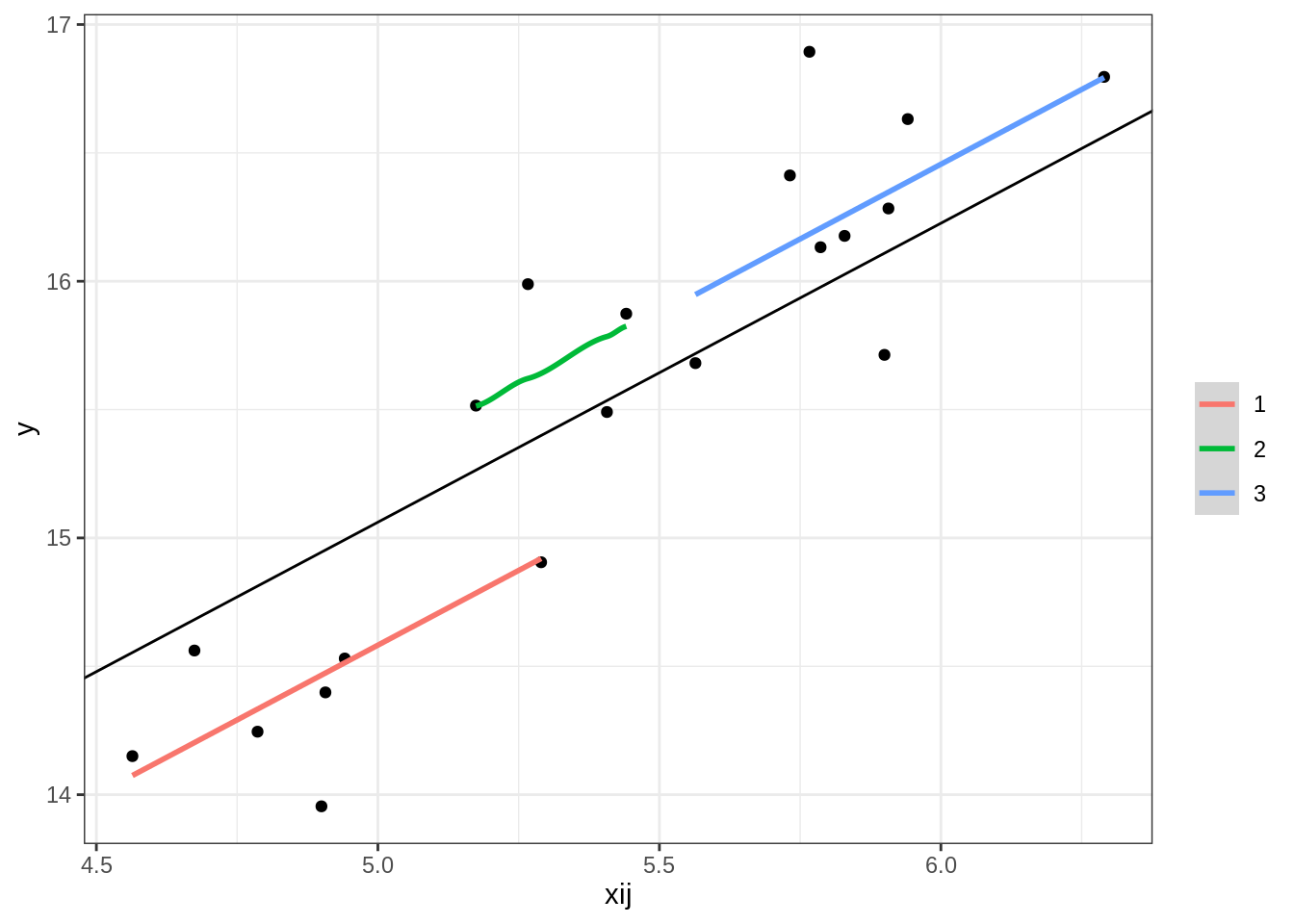
A good lecture to view can be found here.
Computing studentized (conditional) residuals
Studentized conditional residuals can be computed as:
\[r_{c, stud} = \frac{r_{cond}}{\sqrt{Var(r_c)}}\]
Computing \(Var(r_c) = K(V-Q)K'\) where \(Q = X(X'V^{-1}X)^{-1}X'\) and \(K = I - ZGZ'V^{-1}\) (See Gregoire et al., 1995, p. 144 and the documentation of the redres package). (It took me a while finding these references!)
getV <- function(x){
  var.d <- crossprod(getME(x, "Lambdat"))
  Zt <- getME(x, "Zt")
  vr <- sigma(x)^2
  var.b <- vr * (t(Zt) %*% var.d %*% Zt)
  sI <- vr * Matrix::Diagonal(nobs(x)) #for a sparse matrix
  var.y <- var.b + sI
}

Vm <- getV(m1)
Qm <- X %*% solve(t(X) %*% solve(Vm) %*% X) %*% t(X)
The \(G\) matrix here is the random effects matrix and \(I\) is an identity matrix.
Gm <- diag(T00, 3) #this is for a random intercept model with 3 clusters
ns <- nobs(m1) #how many observations
Im <- diag(ns)
Km <- Im - z %*% Gm %*% t(z) %*% solve(Vm)
var_rcm <- diag(Km %*% (Vm - Qm) %*% t(Km))
resid(m1) / sqrt(var_rcm) # computing the studentized residuals
1 2 4 6 7 8
-1.683948120 1.221061289 0.268621673 0.054641174 -0.248705949 -0.053740351
9 12 13 16 17 21
-0.292790104 0.006429117 1.286554117 0.172309523 -1.031596290 -2.034238026
23 24 25 26 27 28
2.306557736 -0.905866125 0.876227868 0.797867472 -0.207656765 0.009806903
29 30
-0.241611485 -0.259127850 rstudent(m1) #automatic, using a function 1 2 4 6 7 8
-1.683948120 1.221061289 0.268621673 0.054641174 -0.248705949 -0.053740351
9 12 13 16 17 21
-0.292790104 0.006429117 1.286554117 0.172309523 -1.031596290 -2.034238026
23 24 25 26 27 28
2.306557736 -0.905866125 0.876227868 0.797867472 -0.207656765 0.009806903
29 30
-0.241611485 -0.259127850 References:
Gregoire, T. G., Schabenberger, O., & Barrett, J. P. (1995). Linear modelling of irregularly spaced, unbalanced, longitudinal data from permanent-plot measurements. Canadian Journal of Forest Research, 25(1), 137-156.
— END