Fun with residuals

Random stuff II: Plotting residuals

I was poking around my old teaching files and I found an old file and I wasn’t sure what it was:

dat <- read.table("https://raw.githubusercontent.com/flh3/pubdata/main/Stefanski_2007/mizzo_1_data_yx1x5.txt")
head(dat)

##         V1         V2        V3         V4        V5         V6
## 1 -0.22391  0.0054599  0.380310  0.0135140  0.209240  0.1467100
## 2  0.84413  0.1073700 -0.026533  0.0458640  0.012987 -0.0271900
## 3  1.06240  0.0911160  0.181260  0.0501710 -0.188670 -0.0120820
## 4 -1.04170  0.4404900  0.245960  0.0054154 -0.212920  0.1015200
## 5  0.15655 -0.1705100  0.147620  0.0836320 -0.095286 -0.0078451
## 6 -0.13526  0.0616050 -0.804130 -0.0259500  0.291730 -0.0783840

dim(dat)

## [1] 3785    6

Turns out it was an old data file I had used in class discussing regression diagnostics. We often talk about the assumption of the homoskedasticity of residuals and we graphically depict that by plotting the fitted values on the X axis and the residuals on the y axis. If all is well, we are told that we should have any discernible pattern.

So this is a dataset of 3,785 observations and 6 variables. We can predict the first variable (V1) using all the other variables in the dataset (V2 to V6).

m1 <- lm(V1 ~ ., data = dat)

If we plot the residuals, we get:

plot(fitted(m1), resid(m1))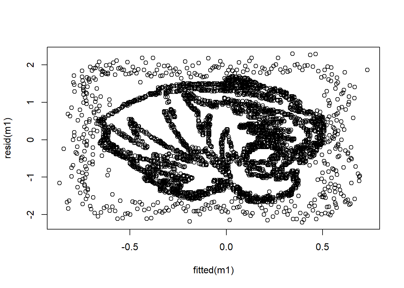

Just thought that was neat. This is based on the work of:

Stefanski, L. A. (2007). Residual (sur)realism. The American Statistician, 61(2), 163-177. https://doi.org/10.1198/000313007X190079

I can’t find the original website where this came from but definitely check out the paper!

Here’s the original image:

Figure 1: MU TIGERS

– END