Years ago I had written a post on using multiple imputation, weights, and accounting for clustering using R. However, the process was actually quite cumbersome and now in 2024, there are more straightforward ways of handling this.
1. Load in the required packges
library(dplyr) #for basic data management
library(tidyr) #converting wide to tall
library(estimatr) #estimating models with robust SEs
library(mitml) #for imputation and analyzing MI datasets
library(MLMusingR) #contains the sample dataset
library(mice) #for carrying out the analysis with MI data
library(modelsummary) #outputting the results nicely
library(survey) #alternative (classic) way
2. Load in the dataset
We will use the pisa2012 dataset in the MLMusingR package. Abbreviated version of the full dataset consisting of 3,136 students in 157 schools. There is no missing data.
data(pisa2012)
names(pisa2012)
[1] "pv1math" "pv2math" "pv3math" "pv4math" "pv5math" "escs"
[7] "schoolid" "st29q03" "st04q01" "w_fstuwt" "w_fschwt" "sc14q02"
[13] "pwt1" "noise1" dplyr::n_distinct(pisa2012$schoolid) #length(table(pisa2012$schoolid))[1] 157nrow(pisa2012)[1] 31363. Create some missing data
Randomly create some missing data in this dataset…
set.seed(123)
sel <- rbinom(nrow(pisa2012), 1, plogis(-2 - scale(pisa2012$pv1math)))
sel2 <- sample(nrow(pisa2012), 300)
dat <- pisa2012 #copy data
dat <- mutate(dat, escs = ifelse(sel == 1, NA, escs))
dat$st04q01[sel2] <- NA
mice::md.pattern(dat, rotate.names = TRUE)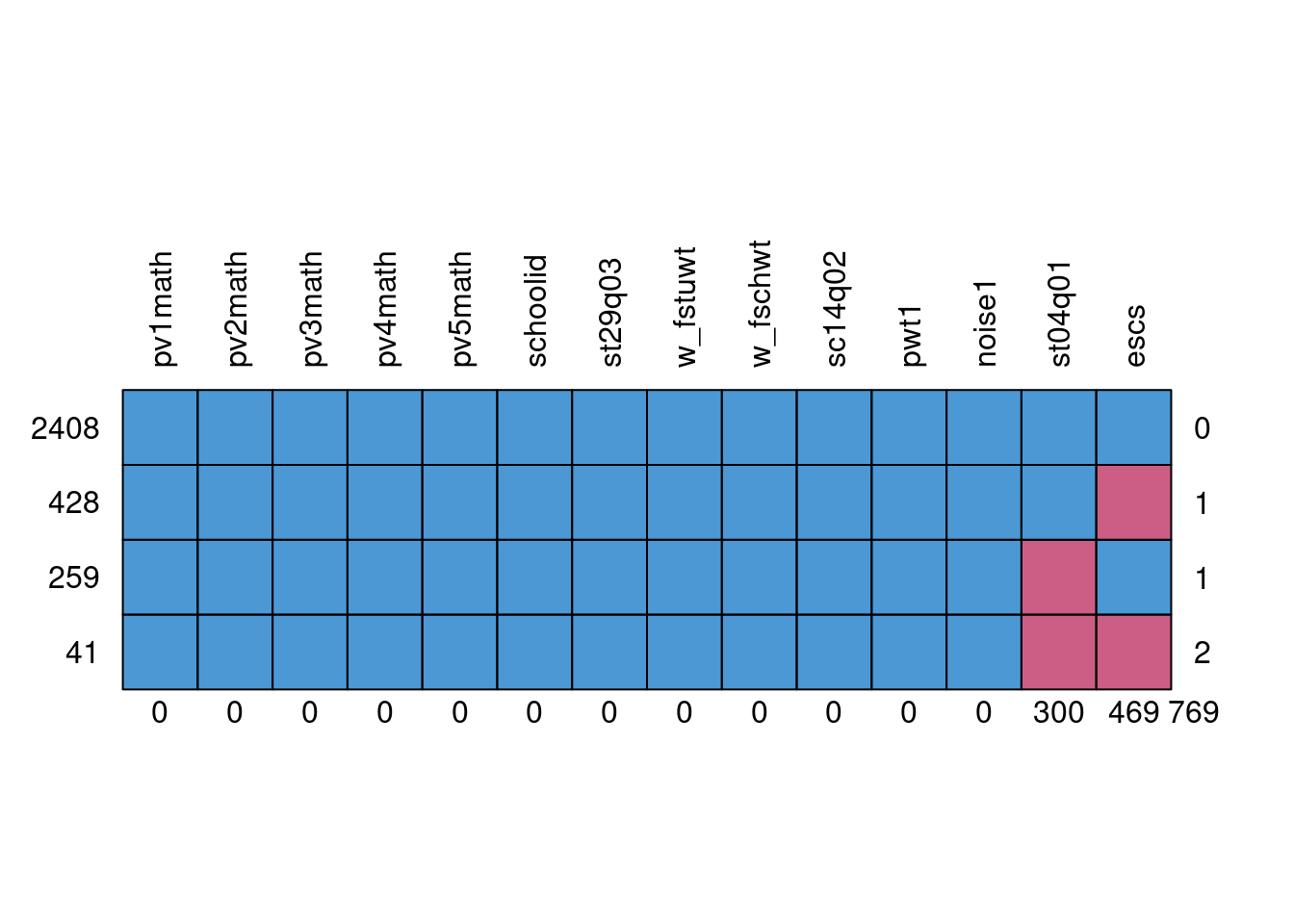
     pv1math pv2math pv3math pv4math pv5math schoolid st29q03 w_fstuwt w_fschwt
2408       1       1       1       1       1        1       1        1        1
428        1       1       1       1       1        1       1        1        1
259        1       1       1       1       1        1       1        1        1
41         1       1       1       1       1        1       1        1        1
           0       0       0       0       0        0       0        0        0
     sc14q02 pwt1 noise1 st04q01 escs
2408       1    1      1       1    1   0
428        1    1      1       1    0   1
259        1    1      1       0    1   1
41         1    1      1       0    0   2
           0    0      0     300  469 769
Now, 65% of the data are complete.
As an example (to show differences), just run a basic regression using lm_robust that uses weights and accounts for clustering:
## testing, just one pv
m1 <- lm_robust(pv1math ~ sc14q02 + st29q03 + st04q01 + escs,
                cluster = schoolid,
                weights = w_fstuwt,
                data = pisa2012)
m2 <- update(m1, data = dat)
Nicely output the summary using modelsummary:
msummary(list('comp' = m1, 'wmis' = m2), stars = TRUE)| comp | wmis | |
|---|---|---|
| (Intercept) | 489.614*** | 502.393*** |
| (6.727) | (6.703) | |
| sc14q02Very little | −8.260 | −9.013 |
| (8.202) | (7.691) | |
| sc14q02To some extent | −21.390* | −21.625* |
| (8.925) | (8.951) | |
| sc14q02A lot | −24.347** | −21.216 |
| (8.522) | (13.211) | |
| st29q03Agree | −8.979 | −14.643* |
| (6.070) | (6.816) | |
| st29q03Disagree | −12.354* | −14.143* |
| (6.246) | (6.088) | |
| st29q03Strongly disagree | −35.615*** | −39.421*** |
| (7.088) | (6.995) | |
| st04q01Male | 8.800* | 12.051*** |
| (3.438) | (3.579) | |
| escs | 35.962*** | 33.527*** |
| (1.770) | (1.860) | |
| Num.Obs. | 3136 | 2408 |
| R2 | 0.180 | 0.178 |
| R2 Adj. | 0.178 | 0.175 |
| AIC | 36679.3 | 27943.6 |
| BIC | 36739.8 | 28001.5 |
| RMSE | 80.21 | 76.98 |
| Std.Errors | by: schoolid | by: schoolid |
| + p < 0.1, * p < 0.05, ** p < 0.01, *** p < 0.001 |
Results show some differences. Now, we can impute some data.
4. Create several (m) imputed datasets
NOTE: this is just an example and we are just imputing a few datasets (m = 5) with minimal burn-ins and iterations (just to make this fast). In actuality, we should do this carefully (with more datasets) and perform diagnostics.
We need to get rid of unused factor levels too (using droplevels) to make this run properly.
dat$st04q01 <- droplevels(dat$st04q01)
dat$st29q03 <- droplevels(dat$st29q03)
fml <- list(escs + st04q01 ~ st29q03 + pv1math + pv2math +
    pv3math + pv4math + pv5math + (1|schoolid),
    sc14q02 ~ 1)
imp <- jomoImpute(data = dat, formula = fml, m = 5,
                  n.burn = 100, n.iter = 10,
                  seed = 12345)
Running burn-in phase ...
Creating imputed data set ( 1 / 5 ) ...
Creating imputed data set ( 2 / 5 ) ...
Creating imputed data set ( 3 / 5 ) ...
Creating imputed data set ( 4 / 5 ) ...
Creating imputed data set ( 5 / 5 ) ...
Done!5. Run the Analysis
After imputing the datasets, we can run multiple analyses. First extract the data, then can use the with function to conduct the analyses using the MI datasets. I just use lm_robust since it automatically computes the cluster robust standard errors. NOTE: I just put se_type as an option to make the output closer to the default of the survey package (w/c uses Taylor series linearization). I wouldn’t generally bother and just leave it using the default CR2 standard error (I think the stata option defaults to the CR1 (or HC1) option.) CR2 is probably better anyway.
comp <- mitmlComplete(imp) #extract imputed datasets
m3 <- with(comp, lm_robust(pv1math ~ sc14q02 + st29q03 + st04q01 + escs,
                           cluster = schoolid,
                           weights = w_fstuwt,
                           se_type = 'stata')
) # it works
summary(pool(m3)) #in mice
term estimate std.error statistic df
1 (Intercept) 489.852603 6.805191 71.982193 151.0527
2 sc14q02Very little -8.119152 7.716148 -1.052229 153.5280
3 sc14q02To some extent -19.173837 8.308226 -2.307814 152.7326
4 sc14q02A lot -27.129784 7.425449 -3.653622 103.3223
5 st29q03Agree -9.961652 6.101269 -1.632718 153.3389
6 st29q03Disagree -13.244478 6.267810 -2.113095 153.3487
7 st29q03Strongly disagree -35.568477 6.978400 -5.096939 150.6255
8 st04q01Male 9.574434 3.395175 2.820012 134.8650
9 escs 36.604406 1.762852 20.764306 147.3206
p.value
1 8.279482e-119
2 2.943480e-01
3 2.235188e-02
4 4.081765e-04
5 1.045801e-01
6 3.621177e-02
7 1.020852e-06
8 5.527054e-03
9 1.330509e-45## using survey / just testing on one dataset
formi <- mitools::imputationList(comp)
des <- svydesign(ids = ~schoolid, data = formi, weights = ~w_fstuwt)
m4 <- with(des, svyglm(pv1math ~ sc14q02 + st29q03 + st04q01 + escs))
summary(pool(m4)) term estimate std.error statistic df
1 (Intercept) 489.852603 6.796616 72.073010 143.24832
2 sc14q02Very little -8.119152 7.706326 -1.053570 145.55767
3 sc14q02To some extent -19.173837 8.297690 -2.310744 144.81175
4 sc14q02A lot -27.129784 7.416912 -3.657828 99.14192
5 st29q03Agree -9.961652 6.093510 -1.634797 145.37980
6 st29q03Disagree -13.244478 6.259839 -2.115786 145.38903
7 st29q03Strongly disagree -35.568477 6.969619 -5.103361 142.85224
8 st04q01Male 9.574434 3.391051 2.823441 128.33174
9 escs 36.604406 1.760655 20.790223 139.79835
p.value
1 1.941158e-114
2 2.938257e-01
3 2.225889e-02
4 4.095286e-04
5 1.042551e-01
6 3.606737e-02
7 1.045852e-06
8 5.509562e-03
9 1.305299e-44Results are similar with each other.
6. Accounting for plausible values
If you have plausible values (PVs), which is common with the use of LSAs, we need to combine the imputed datasets x the number of PVs. To do that, we can convert the wide dataset into a long (or tall) dataset. A new imputation number needs to be made which can be just the PV number x the imputation number. To learn more about PVs, can read this post.
ns <- nrow(comp[[1]])
ms <- length(comp)
dat3 <- do.call(rbind, comp)
dat3$.imp <- rep(1:ms, each = ns)
tall2 <- pivot_longer(dat3, col = pv1math:pv5math, names_to = 'type',
                      values_to = 'math')
#tall2$.pv <- readr::parse_number(tall2$type) #extract pv number
tall2$.imp2 <- paste0(tall2$.imp, '_', tall2$type) #pv x m
comp2 <- split(tall2, tall2$.imp2)
comp2 <- as.mitml.list(comp2)

m4 <- with(comp2, lm_robust(math ~ sc14q02 + st29q03 +
 st04q01 + escs,
 cluster = schoolid,
 weights = w_fstuwt)
) # it works
summary(pool(m4))
term estimate std.error statistic df p.value
1 (Intercept) 491.076573 6.934880 70.812552 45.73261 2.157958e-48
2 sc14q02Very little -9.625605 8.175213 -1.177413 49.93955 2.446115e-01
3 sc14q02To some extent -20.485569 8.439116 -2.427454 49.94985 1.885263e-02
4 sc14q02A lot -29.280150 7.447978 -3.931288 40.16962 3.253493e-04
5 st29q03Agree -10.096298 6.246304 -1.616364 47.16816 1.126853e-01
6 st29q03Disagree -13.522595 6.738041 -2.006903 44.90554 5.080290e-02
7 st29q03Strongly disagree -33.654285 7.088381 -4.747810 45.49903 2.078306e-05
8 st04q01Male 8.983724 3.341756 2.688324 43.08784 1.016832e-02
9 escs 36.597545 1.787528 20.473831 48.47028 1.665732e-25#modelsummary(pool(m4), stars = TRUE) #will also workCan also compare to pooled results using testEstimates– the degrees of freedom methods though just differ.
testEstimates(m4) #in mitml
Call:

testEstimates(model = m4)

Final parameter estimates and inferences obtained from 25 imputed data sets.

                          Estimate Std.Error   t.value        df   P(>|t|)       RIV       FMI
(Intercept)                491.077     6.935    70.813 3.357e+03     0.000     0.092     0.085
sc14q02Very little          -9.626     8.175    -1.177 1.300e+05     0.239     0.014     0.014
sc14q02To some extent      -20.486     8.439    -2.427 1.338e+05     0.015     0.014     0.013
sc14q02A lot               -29.280     7.448    -3.931 8.534e+02     0.000     0.201     0.170
st29q03Agree               -10.096     6.246    -1.616 6.310e+03     0.106     0.066     0.062
st29q03Disagree            -13.523     6.738    -2.007 2.532e+03     0.045     0.108     0.098
st29q03Strongly disagree   -33.654     7.088    -4.748 3.085e+03     0.000     0.097     0.089
st04q01Male                  8.984     3.342     2.688 1.541e+03     0.007     0.143     0.126
escs                        36.598     1.788    20.474 1.508e+04     0.000     0.042     0.040

Unadjusted hypothesis test as appropriate in larger samples.
Results can be compared again to results using the survey package. We do not need to convert the dataset to a tall format and instead, I use the withPV function in the mitools package. NOTE how this is done (the notation used may just be a bit cumbersome).
#formi <- mitools::imputationList(comp)
des <- svydesign(ids = ~schoolid, #strata = ~strat,
 weights = ~w_fstuwt,
 data = formi)

library(mitools)
t1 <- with(des,
 fun = function(a_design){
 withPV(list(math ~ pv1math + pv2math +
 pv3math + pv4math + pv5math),
 data = a_design,
 action = quote(survey::svyglm(math ~ sc14q02 + st29q03 +
    st04q01 + escs,
 design = .DESIGN)),
 rewrite = FALSE)
 }
)

# to combine over PVs within an imputation
result <- lapply(t1, MIcombine)

# to combine over imputations
summary(MIcombine(result))
Multiple imputation results:
MIcombine.default(result)
results se (lower upper) missInfo
(Intercept) 491.076573 7.005072 477.346278 504.8068667 1 %
sc14q02Very little -9.625605 7.896699 -25.102888 5.8516789 0 %
sc14q02To some extent -20.485569 8.152751 -36.464894 -4.5062434 1 %
sc14q02A lot -29.280150 7.008454 -43.066946 -15.4933544 12 %
st29q03Agree -10.096298 6.285855 -22.416403 2.2238062 0 %
st29q03Disagree -13.522595 6.811890 -26.873698 -0.1714927 0 %
st29q03Strongly disagree -33.654285 7.157328 -47.683179 -19.6253900 1 %
st04q01Male 8.983724 3.407352 2.301362 15.6660854 5 %
escs 36.597545 1.771980 33.123908 40.0711819 2 %END