Omitted Variable Bias (OVB) Example
Omitted Variable Bias (OVB) Example
Jun 26, 2018
·
3 min read
Illustrates why OVB is an issue
This issue plagues a lot of the analysis using secondary or observational data
- Data are already existing
- We may have unobserved characteristics that were not collected
To illustrate how OVB may affect regression results, we examine some simulated data.
Create some correlated data
library(stargazer) #to create simpler regression output
library(gendata) #to simulate data
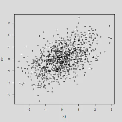
#1 create two correlated variables X1 and X2 (r = .50)
dat <- genmvnorm(k = 2, .5, n = 1000, seed = 123)
cor(dat)
##       X1    X2
## X1 1.000 0.488
## X2 0.488 1.000
Plot of the correlated variables
plot(dat)
Create Y through this data generating process
B1 <- 3
B2 <- 5
set.seed(1234) #add seed so the error is the same
dat$Y <- dat$X1 * B1 + dat$X2 * B2 + rnorm(1000) #add error
#coefficient for B1 = 3 and B2 = 5
Run some regressions
B1 should be 3 and B2 should be 5.
m1 <- lm(Y ~ X1 + X2, data = dat)
summary(m1) #correct
##
## Call:
## lm(formula = Y ~ X1 + X2, data = dat)
##
## Residuals:
##    Min     1Q Median     3Q    Max
## -3.296 -0.656 -0.012  0.637  3.202
##
## Coefficients:
##             Estimate Std. Error t value Pr(>|t|)
## (Intercept)  -0.0265     0.0316   -0.84      0.4
## X1            3.0437     0.0377   80.66   <2e-16 ***
## X2            5.0062     0.0350  143.10   <2e-16 ***
## ---
## Signif. codes:  0 '***' 0.001 '**' 0.01 '*' 0.05 '.' 0.1 ' ' 1
##
## Residual standard error: 0.997 on 997 degrees of freedom
## Multiple R-squared:  0.981,	Adjusted R-squared:  0.98
## F-statistic: 2.51e+04 on 2 and 997 DF,  p-value: <2e-16
What about if we ‘forget’ or omit X1 or X2?
m2 <- lm(Y ~ X1, data = dat)
m3 <- lm(Y ~ X2, data = dat)
#export_summs(m1, m2, m3)
Compare models side by side:
stargazer(m1, m2, m3, type = 'text', no.space = T,
                     star.cutoffs = c(.05, .01, .001),
                     keep.stat = c("n","rsq"))
##
## ============================================
##                    Dependent variable:
##              -------------------------------
##                             Y
##                 (1)        (2)        (3)
## --------------------------------------------
## X1            3.040***   5.680***
##               (0.038)    (0.153)
## X2            5.010***             6.380***
##               (0.035)               (0.084)
## Constant       -0.026     0.169     -0.097
##               (0.032)    (0.146)    (0.087)
## --------------------------------------------
## Observations   1,000      1,000      1,000
## R2             0.981      0.580      0.853
## ============================================
## Note:          *p<0.05; **p<0.01; ***p<0.001
Notice
- How strong the bias is when the variables are correlated with each other
- Notice how different the coefficients are in models 2 and 3
- The bias will change based on the strength of the correlation and the direction of the correlation
If the variables are not correlated with each other
- Will not be an issue
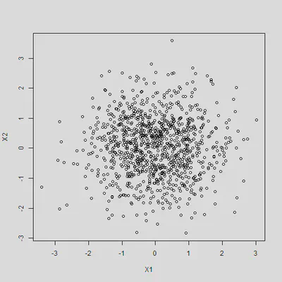
set.seed(541)
X1 <- rnorm(1000)
X2 <- rnorm(1000)
Y <- X1 * B1 + X2 * B2 + rnorm(1000)
By construction, X1 and X2 are not correlated with each other
cor(X1, X2)
## [1] 0.00236
plot(X1, X2)
Results will not be biased
m4 <- lm(Y ~ X1 + X2)
m5 <- lm(Y ~ X1)
m6 <- lm(Y ~ X2)
stargazer(m4, m5, m6, type = 'text', no.space = T,
                     star.cutoffs = c(.05, .01, .001),
                     keep.stat = c("n","rsq"))
##
## ============================================
##                    Dependent variable:
##              -------------------------------
##                             Y
##                 (1)        (2)        (3)
## --------------------------------------------
## X1            3.000***   3.010***
##               (0.031)    (0.159)
## X2            4.980***             4.990***
##               (0.032)               (0.101)
## Constant       0.0003     0.301     -0.010
##               (0.031)    (0.159)    (0.100)
## --------------------------------------------
## Observations   1,000      1,000      1,000
## R2             0.972      0.263      0.711
## ============================================
## Note:          *p<0.05; **p<0.01; ***p<0.001
This is also a reason why experiments use random assignment
- Due to randomization, X (or the treatment assignment variable) will not be related to the error term
- Two groups will be the ‘same’ on both observed and unobserved characteristics (with happy randomization)
- Notice as well the differences in the standard errors (much smaller in the full model)