Why does centering reduce multicollinearity?

Last updated on Jan 21, 2023 3 min read centering

Centering often reduces the correlation between the individual variables (x1, x2) and the product term (x1 $\times$ x2). In the example below, r(x1, x1x2) = .80. With the centered variables, r(x1c, x1x2c) = -.15.

NOTE: For examples of when centering may not reduce multicollinearity but may make it worse, see EPM article.

set.seed(123)
x1 <- rnorm(100, 10, 1)
x2 <- rnorm(100, 15, 1) 
x1x2 <- x1*x2
x1c <- x1 - mean(x1)
x2c <- x2 - mean(x2)
x1x2c <- x1c * x2c
dat <- data.frame(x1, x2, x1x2, x1c, x2c, x1x2c)
round(cor(dat), 2)

##          x1    x2  x1x2   x1c   x2c x1x2c
## x1     1.00 -0.05  0.80  1.00 -0.05 -0.15
## x2    -0.05  1.00  0.55 -0.05  1.00 -0.17
## x1x2   0.80  0.55  1.00  0.80  0.55 -0.17
## x1c    1.00 -0.05  0.80  1.00 -0.05 -0.15
## x2c   -0.05  1.00  0.55 -0.05  1.00 -0.17
## x1x2c -0.15 -0.17 -0.17 -0.15 -0.17  1.00

A question though may be raised why centering reduces collinearity?

Consider the basic equation for a correlation:

$r_{(X, Y)} = \frac{c o v (X, Y)}{\sqrt{(v a r (X) \cdot v a r (Y))}}$

For the product score (X1X2) and X1:

$r_{(X 1 X 2, X 1) = \frac{c o v (X 1 X 2, X 1)}{\sqrt{(v a r (X 1 X 2) \cdot v a r (X 1))}}}$

Focusing only on the numerator and using covariance algebra, the covariance of a product score (X1X2) with another variable (X1) can be written as:

$c o v (A B, C) = E (A) \cdot c o v (B, C) + E (B) \cdot c o v (A, C)$ $= E (X 1) \cdot c o v (X 2, X 1) + E (X 2) \cdot c o v (X 1, X 1)$ $= E (X 1) \cdot c o v (X 2, X 1) + E (X 2) \cdot v a r (X 1)$

With mean-centered variables:

$r_{((X 1 - \bar{X} 1) (X 2 - \bar{X} 2), (X 1 - \bar{X} 1))} = \frac{c o v ((X 1 - \bar{X} 1) (X 2 - \bar{X} 2), (X 1 - \bar{X} 1))}{\sqrt{v a r ((X 1 - \bar{X} 1) (X 2 - \bar{X} 2)) \cdot v a r ((X 1 - \bar{X} 1))}}$

Focusing only on the numerator again:

$= E (X 1 - \bar{X} 1) \cdot c o v (X 2 - \bar{X} 2, X 1 - \bar{X} 1) + E (X 2 - \bar{X} 2) \cdot c o v (X 1 - \bar{X} 1, X 1 - \bar{X} 1)$ $= E (X 1 - \bar{X} 1) \cdot c o v (X 2 - \bar{X} 2, X 1 - \bar{X} 1) + E (X 2 - \bar{X} 2) \cdot v a r (X 1 - \bar{X} 1)$

The expected value though of a mean centered variable is zero. So if the numerator is zero, the whole equation reduces to zero (on average).

$= 0 \cdot c o v (X 2 - \bar{X} 2, X 1 - \bar{X} 1) + 0 \cdot v a r (X 1 - \bar{X} 1)$

Using a short simulation

Randomly generate 100 x1 and x2 variables
Mean center the variables
Compute corresponding interactions (x1x2 and x1x2c)
Get the correlations of the variables and the product term (r is for the raw variables, cr is for the centered variables)
Get the average of the terms over the replications

set.seed(4567)
reps <- 1000
r1 <- r2 <- cr1 <- cr2 <- numeric(reps)
for (i in 1:reps){
  x1 <- rnorm(100, 10, 1) #mean of 10, SD = 1
  x2 <- rnorm(100, 15, 1) #mean of 15, SD = 1 
  x1x2 <- x1*x2
  x1c <- x1 - mean(x1)
  x2c <- x2 - mean(x2)
  x1x2c <- x1c * x2c
  cr1[i] <- cor(x1c, x1x2c)
  cr2[i] <- cor(x2c, x1x2c)
  r1[i] <- cor(x1, x1x2)
  r2[i] <- cor(x2, x1x2)
}

# r(x1,x2) should be zero because generated independently
res <- data.frame(r1, r2, cr1, cr2)
round(colMeans(res), 3)

##     r1     r2    cr1    cr2 
##  0.829  0.551 -0.001  0.008

On average, the correlations of the centered variables are 0 or near 0. They are not always zero and plotting the distribution shows the range of correlations.

library(dplyr)
library(tidyr)
library(ggplot2)
mm <- gather(res, key = 'vars', value = 'r')
mm %>% ggplot(aes(x = r)) +
  geom_histogram(bins = 60) + facet_grid(~vars) +
  theme_bw()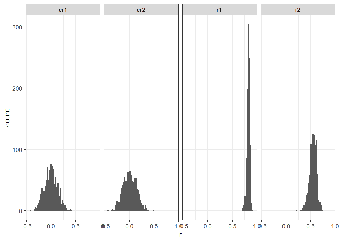

– END

centering