🧪Analyzing dosage effects using an instrumental variable approach to handle noncompliance in RCTs💉
Posted: Jul 28, 2026
A plain-language guide, with a worked R example
This is based on:
Huang, F. L. (2026). Using fidelity of implementation data in randomized controlled trials: A primer on using instrumental variables in educational research. The Journal of Experimental Education. https://www.tandfonline.com/doi/full/10.1080/00220973.2026.2672864
If you’ve ever run (or read about) a randomized controlled trial in education, you’ve probably run into this problem: not everyone assigned to the treatment group actually does (or takes) the treatment, and sometimes people in the control group get a bit of it too. This is called noncompliance, and it’s the norm rather than the exception.
The usual (and usually incorrect) way researchers handle this is to just compare the outcomes of people who actually did (or took) the program against everyone else, treatment or control. The problem is that people who show up and fully participate are probably different in other ways too — more motivated, more organized, whatever — and those same traits could independently improve their outcomes. So the comparison is contaminated by a hidden confound.
Instrumental variable (IV) estimation offers a clean way around this, and — conveniently — an RCT hands you the instrument for free: the random assignment itself.
NOTE: IV estimation is “standard fare” in econometrics classes. In econometerics books, usually a chapter or two is dedicated to the topic. However, in education and psychology methods books, IVs are almost never mentioned (not unless written by someone with an econometrics background or a book on estimating causal effects). NOTE: I use IV to refer to instrumental variables– not independent variables.
The core idea
Picture three variables:
- Z — treatment assignment (randomized: 1 = assigned to treatment, 0 = assigned to control)
- T — treatment take-up (did they actually participate? 1 = yes, 0 = no)
- Y — the outcome of interest
If everyone complied perfectly, Z and T would be identical, and you could just compare outcomes directly. With noncompliance, Z and T diverge, and some unmeasured factor (call it U) may be driving both take-up and the outcome.
The trick: because Z was randomly assigned, it’s guaranteed to be unrelated to that confound U. So instead of asking “what’s the effect of T on Y,” we ask “how much does Z move T, and how much does Z move Y” — then take the ratio. That ratio is called the Wald estimator, and it isolates the causal effect of treatment take-up for the people whose behavior was actually changed by their assignment (the “compliers”).
The IV pathway
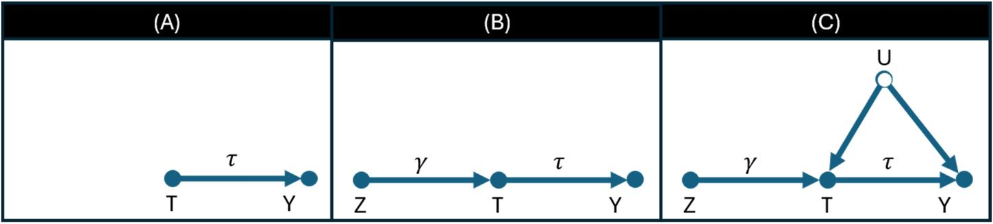
The causal story breaks into three pieces:
- Z → T (the “compliance rate”): does being assigned to treatment actually make someone take it? In an RCT this is almost guaranteed — you can’t get 0% take-up after actively assigning people to a program (not unless you’ve done something really wrong).
- T → Y (the effect you actually want): does taking the treatment change the outcome?
- U → T and U → Y: an unmeasured confounder — like motivation — that influences both whether someone participates and how well they do. This is what makes a naive “compare participants to everyone else” comparison biased.
Because Z was randomly assigned, it’s mathematically guaranteed to be unrelated to U. That’s what makes Z a valid instrument: it moves T, but has no back-door connection to Y other than through T. This last condition — that assignment affects the outcome only through participation, with no direct shortcut — is called the exclusion restriction, and in most RCTs it holds by design (assignment alone shouldn’t improve test scores; actually attending the program should).
With that in place, you don’t need to observe U at all. You can recover the causal effect using just the ratio of two observable quantities: the intention-to-treat effect (Z’s effect on Y) divided by the compliance rate (Z’s effect on T). That ratio is exactly what two-stage least squares regression computes for you.
Two effects worth knowing
- ITT (intention-to-treat): the effect of being assigned to treatment, regardless of whether people actually participated. This is just Y regressed on Z. It’s a valid causal effect — just a diluted one, since it includes people who never engaged. We report this and this of general interest (it is a practical effect).
- CACE (complier average causal effect), also called LATE (the local average treatment effect): the effect of the treatment specifically for the “compliers” — people who took the treatment because they were assigned to it (and wouldn’t have otherwise). This is what IV estimation recovers, and it’s almost always larger than the ITT.
The relationship is simple: ITT = compliance rate × CACE, so CACE = ITT ÷ compliance rate.
The four compliance types
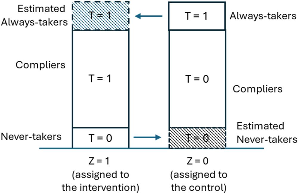
Every participant in a trial falls into one of four types, based on what they’d do if assigned to treatment versus if assigned to control:
| Type | If assigned to treatment | If assigned to control | Can we identify them? |
|---|---|---|---|
| Complier | Takes it | Skips it | Only in aggregate (%) |
| Never-taker | Skips it anyway | Skips it anyway | Yes — directly observable in the treatment group |
| Always-taker | Takes it anyway | Takes it anyway | Yes — directly observable in the control group |
| Defier | Skips it (does opposite) | Takes it (does opposite) | Assumed not to exist |
Two of these types are visible directly in your data:
- Anyone assigned to treatment but who never showed up is a never-taker.
- Anyone assigned to control who got the treatment anyway (a crossover) is an always-taker.
The tricky part is that among the people who did what their assignment predicted (Z=1,T=1 or Z=0,T=0), you can’t tell compliers apart from always-takers or never-takers just by looking at one person. The fix is to lean on randomization itself: since assignment was random, the proportion of never-takers and always-takers should be roughly equal across both arms of the trial. That lets you back out the complier percentage using simple arithmetic, even though you can’t tag each individual.
IV analysis also assumes there are no defiers — nobody who takes the opposite of what they’re told. This is called the monotonicity assumption, and it’s usually reasonable: it just says assignment can only push participation up, never down.
In many school-based interventions, control-group students literally can’t access the program, so there are no always-takers either — this is called one-sided noncompliance, and it’s the simplest case to work with.
When we refer to dosage (or fidelity of implementation), we are talking about the actual amount of treatment received by the participants, as opposed to their assigned dose. Above a certain threshold, we may classify an individual based on a certain compliance type.
Worked example in R
This example is based on an RCT (here using synthetic data) which trained fifth-graders on self-monitoring and self-regulation skills through school counselor–led sessions: 310 students across 14 schools were randomized (158 treatment, 152 control). Randomization was at the student level. The outcome is the “Teachers Who Care” scale score.
Fidelity data showed that 33% of students assigned to treatment never showed up to a single session (never-takers), and since the program wasn’t available to the control group, always-takers can be ruled out — this is a one-sided noncompliance case. In this case, we can use number of sessions as the dosage variable and if a student attended at least one session, we can consider them a complier (note: you can perform sensitivity analyses based on the number of sessions attended; see the paper).
Step 1: Estimate the intention-to-treat (ITT) effect
Regress the outcome on assignment, with covariates, clustering standard errors by school:
library(estimatr)
ex <- rio::import("https://github.com/flh3/pubdata/raw/refs/heads/main/JXE_IV/exiv.rds")
itt <- lm_robust(teachcare_post ~ int + teachcare_pre + fem + frpl + black + other,
                  data = ex, cluster = school_id, fixed_effects = school_id)
summary(itt)
Call:
lm_robust(formula = teachcare_post ~ int + teachcare_pre + fem +
    frpl + black + other, data = ex, clusters = school_id, fixed_effects = school_id)

Standard error type:  CR2

Coefficients:
              Estimate Std. Error t value  Pr(>|t|)  CI Lower CI Upper    DF
int            0.18328    0.07975  2.2982 0.0462083  0.003797  0.36277 9.315
teachcare_pre  0.58589    0.09143  6.4084 0.0002158  0.374718  0.79707 7.925
fem            0.17876    0.04742  3.7699 0.0049753  0.070370  0.28716 8.425
frpl           0.14516    0.07720  1.8803 0.0927318 -0.029453  0.31976 9.010
black         -0.06814    0.07332 -0.9294 0.3780712 -0.235231  0.09894 8.586
other          0.15943    0.08445  1.8879 0.0940230 -0.033743  0.35260 8.389

Multiple R-squared:  0.4595 ,   Adjusted R-squared:  0.4241
Multiple R-squared (proj. model):  0.4152 , Adjusted R-squared (proj. model):  0.3769
F-statistic (proj. model): 53.97 on 6 and 13 DF,  p-value: 1.934e-08
This gives an ITT effect of about 0.18 (statistically significant; in SD units).
Step 2: Estimate the compliance rate
Regress actual participation (takeup) on assignment (int):
first.stage <- lm_robust(takeup ~ int + teachcare_pre + fem + frpl + black + other,
                          data = ex, cluster = school_id, fixed_effects = school_id)
summary(first.stage)
Call:
lm_robust(formula = takeup ~ int + teachcare_pre + fem + frpl +
    black + other, data = ex, clusters = school_id, fixed_effects = school_id)

Standard error type:  CR2

Coefficients:
              Estimate Std. Error t value  Pr(>|t|) CI Lower CI Upper    DF
int            0.66529    0.02604 25.5506 6.080e-10  0.60669  0.72389 9.315
teachcare_pre -0.08186    0.01815 -4.5099 2.024e-03 -0.12379 -0.03993 7.925
fem           -0.02517    0.03510 -0.7172 4.927e-01 -0.10541  0.05506 8.425
frpl           0.07971    0.04134  1.9280 8.592e-02 -0.01380  0.17322 9.010
black         -0.06270    0.03651 -1.7176 1.216e-01 -0.14590  0.02049 8.586
other          0.06827    0.04928  1.3854 2.016e-01 -0.04445  0.18099 8.389

Multiple R-squared:  0.5375 ,   Adjusted R-squared:  0.5072
Multiple R-squared (proj. model):  0.5323 , Adjusted R-squared (proj. model):  0.5017
F-statistic (proj. model): 602.5 on 6 and 13 DF,  p-value: 4.013e-15
The coefficient on int here is the compliance rate — about 0.67,
meaning 67% of students assigned to treatment actually participated.
Step 3: Estimate the CACE with two-stage least squares
Rather than doing the two steps manually, just use iv_robust, which
handles standard errors correctly. The formula has two parts separated
by |: the outcome model first, then the instrument model (same
covariates in both):
iv1 <- iv_robust(teachcare_post ~ takeup + teachcare_pre + fem + frpl + black + other |
                  int + teachcare_pre + fem + frpl + black + other,
                  data = ex, cluster = school_id, fixed_effects = school_id)
summary(iv1)
Call:
iv_robust(formula = teachcare_post ~ takeup + teachcare_pre +
    fem + frpl + black + other | int + teachcare_pre + fem +
    frpl + black + other, data = ex, clusters = school_id, fixed_effects = school_id)

Standard error type:  CR2

Coefficients:
              Estimate Std. Error t value  Pr(>|t|)  CI Lower CI Upper    DF
takeup         0.27549    0.11852  2.3245 0.0442356  0.008761   0.5422 9.315
teachcare_pre  0.60845    0.09235  6.5882 0.0001831  0.394924   0.8220 7.883
fem            0.18570    0.04901  3.7893 0.0049220  0.073495   0.2979 8.344
frpl           0.12320    0.07507  1.6412 0.1357943 -0.047087   0.2935 8.839
black         -0.05087    0.07127 -0.7137 0.4942873 -0.213226   0.1115 8.607
other          0.14062    0.09303  1.5116 0.1671220 -0.071957   0.3532 8.443

Multiple R-squared:  0.4552 ,   Adjusted R-squared:  0.4195
Multiple R-squared (proj. model):  0.4105 , Adjusted R-squared (proj. model):  0.3719
F-statistic (proj. model): 54.15 on 6 and 13 DF,  p-value: 1.895e-08
This gives a CACE of about 0.28 — roughly 55% larger than the ITT of 0.18. That matches the arithmetic: 0.18 ÷ 0.67 ≈ 0.28.
In plain terms: being assigned to the program raised scores by 0.18 points on average across everyone. But among students who actually attended at least one session, the effect of participating was closer to 0.28 points.
A note on reporting
When you write this up, it’s good practice to report both effects together, plus the compliance rate:
The intention-to-treat (ITT) effect was 0.18 (p < .05). Two-stage least squares regression, using random assignment as an instrument for actual participation, produced a complier average causal effect (CACE) of 0.28 (p < .05) — about 55% larger than the ITT, reflecting the effect among the 67% of students who attended at least one session.
Things to keep in mind
- IVs can’t rescue a program that didn’t work. If the ITT isn’t statistically significant, the CACE usually won’t be either — even though it’s numerically larger.
- Clustered data (e.g., students within schools) needs cluster-robust
standard errors — and with fewer than ~40 clusters (common in
school-based RCTs), use the CR2 correction rather than the default,
which
iv_robust’sclusterargument handles for you. - One instrument can only predict one endogenous variable. If you have two different “doses” of noncompliance, one instrument won’t be able to estimate the causal effect.
See the paper for more details and how to estimate the effect using a structural equation modeling or with a Bayesian approach.
Cite as: